Introduction
Knowledge Discovery in Databases (KDD) is the process of searching large volumes of data for the non trivial extraction of implicit, novel, and potentially useful information. Traditional KDD applications require complete access to the data which is going to be analyzed. Nowadays, a huge amount of heterogeneous, complex data resides on different computers which are connected to each other via local or wide area networks (LANs or WANs). Examples comprise of distributed mobile networks, sensor networks or supermarket chains. The increasing demand to scale up algorithms to these massive data sets which are inherently distributed over networks with limited bandwidth and computational resources has led to methods for parallel and distributed data mining. One of the most common approaches for business applications to perform data mining on such massive datasets is to centralize distributed data in a data warehouse on which the data mining techniques are applied. Data warehousing is a widely used technology which integrates data from multiple data sources into a single repository in order to efficiently execute complex analysis queries. However, despite its commercial success, this approach may be impractical or even impossible for certain business settings, for instance:
- When a huge amount of data is frequently produced at different sites and the cost of its centralization cannot scale in terms of communication, storage and computation. For example, call data records of telephonic conversations.
- Whenever data owners cannot or do not want to release information. This could be in order to maintain privacy or because disclosing such information may result in a competitive disadvantage or a considerable loss in commercial value. For example, data mining across banks by the Reserve Bank of India.
Such scenarios call for distributed data mining. Distributed data mining deals with pattern extraction problem. One of the most studied data mining techniques is clustering. The goal of this technique is to decompose or partition a data set into groups such that both intra-group similarity and inter-group dissimilarity are maximized. In particular, clustering is fundamental in knowledge acquisition. It is applied in various fields including data mining, statistical data analysis, compression and vector quantization.
In this thesis, we present CIODD, a cohesive framework for cluster identification and outlier detection for distributed data. The data is either distributed originally because of its production at different locations or is distributed in order to gain a computational speed up. We use a parameter free clustering algorithm to cluster the data at local sites. These clusters are actually the partial results which are communicated in the form of local models to the central server. The central server aggregates these partial results to give a global solution. A feedback loop is then provided to purify and enhance this global solution.
Below we give a brief statement of the problem addressed in the thesis
Given a dataset D of n points distributed across s sites and a central server, find the clusters of the dataset D by communicating minimum information to the central server such that the accuracy of the obtained clusters is comparable to the results obtained using a centralized clustering approach…
Related Work
Clustering
Clustering partitions a dataset into highly dissimilar groups of similar points. The definition of clusters and outliers depends very much on the domain of the dataset. For the sake of clarity, we provide here general definitions quoted in the literature. A cluster is a set of similar points that are highly dissimilar with other points in the dataset. An outlier or a noise point is an observation which appears to be inconsistent with the remainder of the data. Next, we discuss the various clustering algorithms brieûy.
Partitioning techniques
K-means, PAM, CLARA and CLARANS are good examples for clustering based on partitioning techniques. K-means is in fact a very popular clustering algorithm. These clustering algorithms work under the assumption that there is no noise in the dataset, the clusters are spherical-shaped and the points in the cluster follow uniform distribution. They perform well on datasets containing spherical clusters but also do include noise in the cluster results. They cannot identify clusters of irregular shapes and sizes. CURE is another partitioning based clustering technique developed to reduce the effect of noise and identify elliptical shaped clusters. It uses multiple representative points for each cluster to reduce the effect of noise but cannot capture clusters of different densities.
Hierarchical techniques
Clustering algorithms using this technique aim at producing a tree/dendrogram where each node contains a set of data points (a probable cluster). There are two basic approaches for generating a hierarchical clustering:
On the basis of the proximity definition for two clusters, hierarchical clustering algorithms are also classified as
- Single link or MIN
- Complete link or MAX or CLIQUE
- Average
The single link hierarchical algorithm is more suited to identify clusters of irregular shapes. This technique is computationally intensive, sensitive to the presence of noise points scattered between the clusters and fails in the case of clusters with varying densities. Other variations of this technique are the average link and complete link hierarchical algorithms, which are less sensitive to noise but tend to identify clusters of spherical shape. BIRCH is another clustering technique that uses a hierarchical data structure called CF-tree for partitioning the data points in an incremental way. CF-tree is a height-balanced tree, which stores the clustering features. The algorithm requires two parameters as input: branching factor and cluster diameter threshold. The algorithm is sensitive to the order in which the data points are scanned.
Density-based techniques
Examples of this technique are DBSCAN and OPTICS. They consider the density around each point to identify the cluster boundaries and the core cluster points. The close cluster points in a single neighborhood are then merged. OPTICS does not generate a clustering solution; instead it generates an augmented ordering of the points. Given a reachability distance, it generates reachability plots that capture the local density settings around each point. It can be effective for noisy datasets having arbitrary shaped clusters of different sizes and densities. The clustering results for both these algorithms depend largely on the provided parameters. Finding these parameters for both these algorithms is a challenge for the user.
Graph-based approaches
The clustering algorithms based on these approaches are able to keep the structure of data intact. They are able to remember the positions of a point with respect to the other points and thus can help in finding the clusters of arbitrary shapes and sizes very well.
CIODD: A framework for distributed clustering
The proposed framework CIODD uses object distributed data and is a centralized ensemble based method. CIODD is a cohesive framework for cluster identification and outlier detection for object distributed data. From now onwards by distributed data, we refer to object distributed/homogeneous data. The core idea of the framework is to generate independent local models and combine the local models at a central server to obtain global clusters. A feedback loop is then provided from the central site to the local sites to complete and refine the obtained global clusters. We illustrate the CIODD framework in Figure 3.1. The steps involved in the process of distributed clustering for the CIODD framework are:
DD: Data Distribution
As stated earlier, the need for distributed clustering might occur not only when the data is inherently distributed but also when the data cannot be processed using a single processor and thus to gain a computational speed up, it is distributed across multiple processors. The step DD in this process involves the distribution of data across the local sites.
There could be different data partitioning strategies which could be employed for distributed data mining. The one we use is cover based partitioning, i.e. In our approach the partitions are overlapping. Here two partitions D i and D j are over- lapping if | Di ∩ Dj | >0.
Local Clustering Algorithm
The clustering algorithm that we use for clustering the data at local sites is the Stability based RECORD Algorithm (SRA) with minor modifications.
The SRA algorithm uses the notion of k-Reverse Nearest Neighbor (kRNN) and Strongly Connected Components (SCC) to:
- Derive clearly distinguishable clusters, and
- To identify and remove outliers during the process of clustering.
SRA presents a cohesive framework for both cluster analysis and outlier detection that improves the quality of the clustering solutions. Definitions
kRNN (p j): The set of points which consider pj asone of their kth nearest neighbors.
kRNN (p j) =∪i=1p rnn i (p j )
Strongly Connected Components (SCC): TheSCC of a digraph partitions the vertices’s into subsets such that all the points of each subset are mutually reachable.
Core point
In a cluster, a core point is a point that lies amidst the dense set of points of the cluster. The concept of kRNN is used to capture the nature of this neighborhood of the point. For a given value of k, a point having |kRNN|≥ k is flagged as a core point.
Boundary point and Outlier
A boundary point in a cluster is a point which lies in the transition region of dense points to noise points in the cluster. An outlier is a point far from most others in a set of data. Based on large number of experiments done over various datasets, it was found in [11] that an outlier has | kRNNs | < k and most of its kRNNs are outliers. Also for a boundary point, its | kRNNs|< k and most of its kRNNs are core points.
Basic RECORD Algorithm
Stability based RECORD algorithm (SRA) is a hierarchical clustering algorithm which uses the basic RECORD algorithm presented in11. Therefore we first describe the basic RECORD algorithm and then move on to the SRA in the later parts of the section. The major steps involved in the basic RECORD algorithm are as follows:
Step 1-kRNN Computation
Generate the distance matrix based on the distance function d(i, j). Here distance function is a measure to define the distance between two data points. Calculate the kRNN sets of each point as follows:
- For each point p, identify the k-nearest points knn(p). For every point q∈ kNN(p), increase the count of its reverse nearest neighbors by 1.
- Add the directed edge (q∈ kNN (p), p) to the kRNN graph.
Step 2-Outlier detection
For each data point, the numbers of points in kRNN (p) are checked. For any data point p if | kRNN|< k, it is ûagged as an outlier. The point p and all out-going edges from p are removed from the kRNNG graph. After removing all outlier points from the graph, the modified graph is represented as kRNNG > k. Also, we have the graph kRNNG < k which is given by kRNNG – kRNNG > k. This kRNNG > k includes only outlier points and their corresponding out-going edges and is used at later stages to get a stable clustering solution.
For our experiments, we chose l to be 1 and terminate the local clustering algorithm when the number of SCCs remains constant for both the subgraphs for at least two successive values of k.
The first step of the SRA requires the computation of the complete distance matrix to compute the kNN of a data point. This becomes a bottleneck in the performance of the SRA algorithm. In the next subsection, we present an efficient approach to compute these k nearest neighbors of a data point.
Efficient Computation of kNN
For computing the kNN of a point one needs to compute the distance/similarity matrix. A similarity matrix is a n* n matrix of distance measures which expresses the similarity between any two data points. The O(n2) complexity becomes a bottleneck in the performance of the SRA algorithm. The experiments carried out in [11] show that stable clustering solution is found by exploring within 100 neighbors of every data point. Hence we propose an efficient method to compute the kNN of every data point where k has some known value which is much less than n. The basic idea here is to convert the kNN search of a data point from the entire search space to a search in some neighborhood of the point using the property explained in Theorem 1.
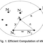
Consider a data point A and its kNN points ordered on distance: N1, N2, . . . , Nk. Let Nk be the kth nearest neighbor of A and d (A, Nk) = x, where d (A, N k) is the distance between A and N k. We define a neighborhood value of a data point with respect to a value k, as the radius of the circle that encompasses its k nearest neighbors. Thus x is the neighborhood value of A.
Theorem 1
Consider any one kNN, Ni of A and let d (A, N i) = y. Then the circle with center as N i and radius x+y, encompasses all the points N1, N2, . . . , Ni-1 ,Ni+1, . . . , Nk and A (refer Figure 4.1).
Proof
Since radius of the circle is x + y and point A is at distance y from Ni, A lies in the circle.
Now consider any kNN of A other than N i say N j. Let d (N i, N j) = w. Then in the (Ni, Nj, A), by triangle inequality w < y + z. Since Nk is the k th nearest neighbor, z < x. Therefore, w < x + y. Thus Nj lies inside the circle. Hence proved.
Based on theorem 1, the working of the kNN computation algorithm is given below.
- Initialize P S and HP S to be empty sets. Here P S is the list of points which are to be processed and HP S is the set of points which are already processed.
- Let d i be any data point whose neighbors are not yet found. Its kNN set {Ni,….. Nk} is computed by determining the distance of d i with every data point. Let NBHd i be the neighborhood value of d i. The kNN set is then added to a processing list P S which is a set of ordered pairs (N i, NBHd ii+ d(N i, d i)) where d(N i, d i) denotes the distance between N i and d i .
- For each pair (T, V )∈ P S, determine all points {P1, . . . , P l} that lie inside the circle that is drawn with T as center and V as radius. Note that l > k by theorem 1. The distance of T from each Pi, ∀i = 1, . . . , l is computed and the kNN set of T, {O1 , . . . , Ok} is determined as the k closest points out of P1, P2, . . . , Pl.
- Let NBHT be the neighborhood value of T. Then the set of pairs (Oi, NBHT + d(T, Oi)) for all i = 1, . . . , k, such that O i is not present in any of the ordered pairs in P S and in HP S, is added to P S. The pair (T, V) is removed from P S and T is added to HP S.
- Step 3 and 4 are repeated until P S becomes empty.
- Repeat step 2, 3, 4 and 5 till the k neighbors for all the data points are found.
Step 3-Cluster Identification
Eliminating outliers from kRNNG results in kRNNG > k. The clusters are now computed based on this kRNNG > k. Each SCC in the kRNNG > k graph becomes a cluster as it follows two rules:
•Each member of the SCC is accepted as k-nearest by at least k points and
•Every possible pair of members in the SCC is mutually reachable depicting the cohesiveness of the graph.
SCCs are also computed on kRNNG < k(sub-graph kRNNG containing only outliers). The SCCs obtained from this graph are clusters of noise points and are very sparse. The SCCs so obtained are used to identify stable clustering solution (Stability based RECORD). An efficient approach to compute these SCCs incrementally is provided in 11.
Step 4-Local outlier incorporation
Since even the boundary points could have their | kRNN |< k, the outlier detection technique discussed above could be very stringent. Because of this, some of the boundary points of the clusters are also identified as outliers. Due to this, the clusters generated are highly dense and incomplete. To avoid such eliminations, after the generation of SCCs, an effort is made to draw each of the outlier points to its nearest cluster. Nearest cluster is the closest majority cluster among kRNN points of the outlier under study. At the end of this step, an outlier point such that majority of its neighbors lie in one cluster, gets ûagged as a cluster point of that cluster.
Stability based RECORD algorithm
Having discussed the basic RECORD algorithm, we now give a brief explanation of the Stability-based RECORD Algorithm (SRA) algorithm. The SRA utilizes the basic RECORDalgorithm, and generates the most stable clustering result as its output. Starting from k = 1, for each value ofk the kRNNG is computed. The kRNNG is split into two subgraphs kRNNG < k and kRNNG <k . SCCs are computed for both the subgraphs. As k increases, the number of SCCs in kRNNG < k and kRNNG > k are checked. After a certain value ofk these numbers do not change. This would imply that no new clusters are formed and no variation in noise behavior is detected. So in [11], the number of SCCs in both the subgraphs is observed for some l consecutive values of k and if they remain constant then the clusters obtained are considered to be stable. The value of l is determined experimentally. For the distributed scenario, the stability constraint has to be less stringent because at any given site only a subset of data is clustered. Because of this, the stability of the clustering algorithm is expected to go down.
The above approach helps us in overcoming the earlier O(n² log n) time complexity of computing the k nearest neighbors for each point. Next we present an analysis of the time complexity of the above approach. We also provide experimental results in which support the obtained worst case bounds on the time spent.
Let SP be the set of points for which the algorithm computes the distance w.r.t all the points in D. For each point in SP, n-1 distance values obtained are sorted to compute the k nearest neighbors. Therefore, the total complexity of this step is s*(n-1)*log(n-1) which is of the order O(s*n*logn). Here | SP | = s. For the remaining points in D- SP, the algorithm calls Expand Neighborhood Search() function. For each point N∈ (D-SP):
I. A region query is issued around N. Let m be the number of points that fall within the region.
II. The distance values of N to each of the neighbors obtained in (i) are computed and sorted.
The complexity of step (i) is O (logn) and that of the second step is O (mlogm). Therefore, the total complexity due to all points in D- SP is O ([n- s]* [logn + mlogm]), (since | D- SP | = n- s). Hence the total complexity due to all points is: O (s*n* logn + (n- s)* [logn + mlogm])
The overall cost for computing the k nearest neighbors can be given as O (c* n* log n + k2 * n* log (n/c)). The experimental results presented in Table 1 show that as the difference between the k value and the size of the dataset i.e. n increases, the efficiency gained by employing the proposed approach also increases.
In the next section, we discuss the information that is communicated to the central server, using which the global clusters can be acquired.
Acquiring the Local Model
After having clustered the data locally at each local site, we would like to communicate to the central server adequate amount of information that will describe the local clustering results. These local models have to be such that they give an accurate description of the local clustering as far as possible.
The information that can be communicated from the local clusters in the form of local model is
- Cluster statistics such as density information and number of data points in the cluster.
- Representative points from the cluster. These could be chosen from the core/dense regions of the cluster and also from the boundary regions of the cluster.
Acquiring the Global Model
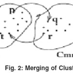
Once the local model from each site is communicated to the central server, a global merging algorithm has to be employed on the local models to acquire the global model. Let there be any two representative SCCs of clusters C ij ( jth cluster from ith site) and Cmn(mth cluster from nth site), which are candidates to be merged. Consider the points p, t∈ Cij and q, r∈ C mn. The clusters C ij and Cmn would merge if for any value k, p∈ kRNN(q) and r∈ kRNN(t) as in Figure 5.1. Here p, q, r, t are the representatives that have been communicated to the central server in the respective local models.
As can be seen, the global merging algorithm is required to cluster the data that is communicated in the form of representatives of the local clusters. At the central server, we again apply the Stability based RECORD algorithm to cluster these local representatives effectively. As stated earlier, the termination condition for the SRA is as follows: the number of SCCs in both the subgraphs (kRNNG<k for the outliers and kRNNG≥k for the core points) are observed for some l consecutive values of k and if they remain constant then the clusters obtained are considered to be stable. The global clusters obtained at this stage might not be complete.
Updation of the global and the local models
After finishing the global clustering, we send the complete global model to all the client sites. Using this information, the client sites can assign each of the objects a label that corresponds to the global cluster to which it belongs.
Results
We conducted the experiments on synthetic datasets and real life datasets to evaluate the efficacy of our approach.
Results for efficient computation of nearest neighbors
In Table 1 we present the results obtained using the approach proposed by us for computing the k nearest neighbors of a data point efficiently. Since the results in [11] show that computing just 100 nearest neighbors is sufficient to get the clusters present in a dataset we take the k value as 100 and show the results for it.
Table 1: Speed up gained in computing the k nearest neighbors
|
Dataset size
|
Ratio T1/T2
|
|
500
|
1.089
|
|
1000
|
2.280
|
|
3000
|
3.373
|
|
5000
|
5.735
|
|
10000
|
9.654
|
|
100000
|
34.173
|
There are two columns in the table1. Column 1 shows the size of the dataset and column 2 shows the ratio T1 /T2. T2 is the time taken by the approach proposed by us in the Section 2.3. T1 is the time taken by the naive approach where to get the k nearest neighbors the entire similarity matrix is computed. As is demonstrated by the results, with the increase in the difference between the k value i.e. 100 and the size of dataset, the efficiency gained by the proposed technique also increases.
Efficacy of the CIODD approach
In this section we discuss the various efficiency and accuracy results obtained for our framework.
Results on synthetic datasets
Syndeca tool set was used to generate synthetic datasets with clusters for experimentation. In order to compute the total time taken by our approach, we carried out the local clustering for all sites and denoted the time taken by these as a set{TLCMi}for i = 1, . . . , s. Here the time taken by the individual sites for this updation phase was denoted by a set{TUM} for i = 1, . . . , s. The overall runtime T for the approach was calculated using the formula given below:
T = T g + max {TLCi}, +max {TUMi}
The variable i spans from 0 to s taking into considerations all the local sites. Here s is the total number of sites, Tg is the time taken by the global merging algorithm GM, T LCMi is the time taken for LCM on the ith site and T UMi is the time taken for the updation phase UM on the ith site.
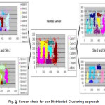
In figure 1 we provide a screen-shot of the results for the Chameleon dataset 1 used in hierarchical clustering. The dataset had 8000 points and six clusters which were very closely spaced and were of various shapes and sizes. The dataset was distributed on four sites. The amount of information communicated as the local models was 10%. As a 1result of the distribution the original clusters were distributed in the form of smaller and sparser clusters and were sent to different local sites. Some of the sites did not even have the complete picture of some clusters with them. As shown in the Figure 2, our approach was able to detect all these clusters accurately after the final phase.
Experiments with real life datasets:
In this section we provide the results for the proposed CIODD framework on three real life datasets. We also provide the performance of the DBDC approach on the same datasets and compare the accuracy results obtained by both. To get the performance results for DBDC, we implemented it in C++. All the experiments were carried out on an AMD dual 64 bit machine with 2 GB of RAM. The evaluation metric that we use for the real life datasets is cluster homogeneity. We define accuracy as:
accuracy = (Σki=0 ai)/n
Here n is the total number of points to be clustered and ai is the number of points that belong to the dominance class of the kth cluster.
Iris Dataset
The Iris flower data set or Fisher’s Iris data set is a multivariate data set introduced by Sir Ronald Aylmer Fisher (1936). The dataset consists of 3 classes, 50 instances each, where each class refers to a type of iris plant namely Iris Setosa, Iris Versicolor, and Iris Verginica. The first class is linearly separable from others while the latter two are not linearly separable. There are four continuous attributes and a target attribute which determines the class of the tuple. The attribute measurement consists of the sepal and petal lengths and widths in cms.
We now present the comparison of CIODD with a distributed clustering algorithm DBDC and three centralized clustering algorithm k- means, DBSCAN and SRA in Table 2. For CIODD and DBDC, we distributed the data on two sites such that each site had 75 points. For the CIODD approach the degree of overlap was kept to be 0 so that the data that is processed by each approach on any site is same. First row in the table corresponds to the number of sites the data was distributed. Since the first three approaches are centralized, the entire data resides on a single site. Next row pertains to the amount of data processedat each site. Third row gives the details about the parameters that are needed to carry out the clustering. Here k, Mpts, Eps, Lpts, LEps, Gpts, GEps refer to number of clusters, minimum points, epsilon, local minimum points, local epsilon, global minimum points and global epsilon respectively. These are the parameters that are required by the k-means, DBSCAN and the DBDC respectively. As stated in [12], we set the global minimum points as 2 and the global epsilon is set twice of the local epsilon.
Also for k- means we kept the k value as 3 since we knew the number of classes beforehand. It can be seen that the SRA and CIODD need no parameters to carry out the local clustering. The next two rows give the number of clusters obtained and the amount of information communicated in various forms to get the results. The last row gives the accuracy calculated using the formula stated above. As can be seen the feedback loop i.e. the UM of the CIODD approach helps it to get a higher accuracy as compared to the accuracy obtained by the DBDC approach. Also the performance of the CIODD approach is comparable to centralized clustering.
Table 2: Results on IRIS dataset
|
|
Kmeans
|
DBSCAN
|
DBDC
|
SRA
|
CIODD
|
|
No. of sites
|
1
|
1
|
2
|
1
|
2
|
|
Dataset size
|
150
|
150
|
75
|
150
|
75
|
|
Parameters
|
K=3
|
Mpts=3
|
LMpts=3
|
None
|
None
|
|
|
|
Eps=0.5
|
LEps=1
|
|
|
|
|
|
|
GMPTS=2
|
|
|
|
|
|
|
GEps=2
|
|
|
|
No.of clusters
|
3
|
10
|
5
|
23
|
6
|
|
Info communicated
|
–
|
–
|
20%
|
–
|
20%
|
|
Accuracy
|
0.667
|
0.5
|
Site1:0.653
|
0.663
|
Site1:0.653
|
|
|
|
|
Site2:0.623
|
|
Site2:0.826
|
|
|
|
|
Final:0.634
|
|
GM:0.733
|
|
|
|
|
|
|
UM:0.812
|
Table 3: Comparison of various distributed clustering approaches
|
Property
|
CIODD
|
SRA
|
DBDC
|
SDBDC
|
DMBC
|
KDEC
|
|
Efficiency
|
yes
|
Yes
|
yes
|
yes
|
Yes
|
Yes
|
|
Clusters of mixed densities
|
yes
|
Yes
|
no
|
no
|
–
|
Yes
|
|
Clusters of varied shapes
|
yes
|
Yes
|
yes
|
yes
|
–
|
–
|
|
Privacy
|
no
|
No
|
no
|
no
|
Yes
|
Yes
|
|
Needs parameters for local
|
no
|
No
|
yes
|
yes
|
Yes
|
–
|
|
clustering
|
|
|
|
|
|
|
|
Amount of info communicated
|
Yes
|
Yes
|
no
|
Yes
|
no
|
yes
|
|
for obtaining global model is tunable
|
|
|
|
|
|
|
|
Detects clusters lost due to
|
yes
|
Yes
|
no
|
no
|
No
|
No (if expected privacy is less, then individual tuples of outliers are sent to complete the global clusters).
|
|
No of rounds of communication
|
2
|
2
|
1
|
1
|
1
|
2
|
Comparison of the existing work with CIODD
As discussed in the earlier sections of the thesis, a distributed clustering algorithm is expected to exhibit several properties.
Conclusions
In this thesis, we present CIODD, a cohesive framework for the identification of clusters and outliers in the distributed environment. The presented framework uses homogeneously distributed data and is a centralized ensemble based method. It requires two rounds of communication between the central server and the local sites. In the first round a global model is obtained from the local models generated as a result of the clustering at local sites. The second round is employed to complete and purify the global clusters obtained in the first round. CIODD uses the parameter free clustering algorithm SRA for the clustering of data at local sites. It also proposes an efficient way to compute the kNN. Unlike previous centralized ensemble based approaches for homogeneousdistributed data, using CIODD, we are able to detect clusters of mixed densities and varied shapes placed in close vicinity of each other. Earlier approaches also fail to handle the local outliers, where as CIODD is able to do so because of the presence of the grid based feedback loop. Moreover, the increase in accuracy obtained due to the introduction of the feedback loop is much more than the increase in the overhead caused by its computation. We also show that without compromising much with the accuracy, the time taken by CIODD is much less than the classical centralized clustering.
For example we were able to cluster a set of 20,000 points by distributing the data on six sites with an accuracy of 98.54% with the amount of information communicated being equal to 9% of the data. Also the time taken by the entire process was 75% less than what was taken by a centralized solution.
Using the results on a synthetic data stream, we show that the CIODD framework might also be used to cluster data streams. Thus, as a part of future work we would like to explore the use of the proposed framework in clustering data streams.
References
- A. K. Jain, M. N. Murthy, and P. J. Flynn., “Data clustering: A review,”
- F. E. Grubbs., “Procedures for detecting outlying observations in samples,” in In Technometrics., pp. 2-21 (1969).
- P. Berkhin., “Survey of clustering data mining techniques.,” in Tech. Report, Accrue Software.
- D. Fasulo., “An analysis of recent work on clustering algorithms: a technical report,”
- S. Guha, R. Rastogi, and K. Shim., “Cure: An efcient clustering algorithm for large databases.” in SIGMOD, (1998).
- T. Zhang, R. Ramakrishnan, and M. Livny, “Birch: An efficient data clustering method for very large databases,” in SIGMOD, (1996).
- M. Ester, H. P. Kriegel, J. Sander, and X. Xu., “A density based algorithm for discovering clusters in large spatial databases with noise.” (1996).
- G. Karypis, E. Han, and V. Kumar, “Chameleon: Hierarchical clustering using dynamic modeling,” Computer, 32(8): 68-75 (1999).
- S. Bandyopadhyay, C. Gianella, U. Maulik, H. Kargupta, K. Liu, and S. Datta, “Clustering distributed data streams in peer-to-peer environments,” Information Science Journal, (2004).
- M. Klusch, S. Lodi, and G. L. Moro, “Distributed clustering based on sampling local density estimates,” in Proceedings of International Joint Conference on Artificial Intelligence (IJCAI 2003), (Mexico), 485-490 (2003).
- S. Vadapalli, S. R. Valluri, and K. Karlapalem, A simple yet effective data clustering algorithm,. ICDM, 2006.
- E. Januzaj, H. P. Kriegel, and M. Pfeiûe, “Towards effective and efficient distributed clustering,” Workshop on Clustering Large Data Sets (ICDM2003), 2003.
- E. Januzaj, H. P. Kriegel, and M. Pfeiûe, “Scalable density-based distributed clustering,” Proc. 8th European Conference on Principles and Practice of Knowledge Discovery in Databases (PKDD), (2004).
- D. K. Tasoulis and M. N. Vrahatis, “Unsupervised distributed clustering,” in In Proceedings of the IASTED International Conference on Parallel and Distributed Computing and Networks. Innsbruck, Austria., (2004.
- S. Guha, N. Mishra, R. Motwani, and L. O’Callaghan, Clustering Data Streams. FOCS.
- “Cluster ensembles – a knowledge reuse framework for combining partitionngs,” pp. 583-617, Journal of Machine learning Research, Dec 2002.
- J. Ghosh, A. Strehl, and S. Merugu, “A consensus framework for integrating distributed clusterings under limited knowledge sharing,” in Proceedings of NSF Workshop on Next Generation Data Mining, pp. 99-108 (2002).
- A. Topchy, A. K. Jain, and W. Punch, “Combining multiple weak clusterings,” pp. 331-338 (2003).
- A. Topchy, B. Minaei-Bidgoli, A. K. Jain, and W. F. Punch, “Adaptive clustering ensembles,” 1: 272-275 (2004).
- A. P. Topchy, M. H. C. Law, A. K. Jain, and A. L. Fred, “Analysis of consensus partition in cluster ensemble,” 225-232 (2004).
- J.R.Vennam and S.Vadapalli, “Syndeca: A tool to generate synthetic datasets for evaluation of clustering algorithms.,” pp. 27-36 COMAD, (2005).

This work is licensed under a Creative Commons Attribution 4.0 International License.