An Aproach of Design and Training of Artificial Neural Networks by Applying Stochastic Search Method
Introduction
This paper is motivated to introduce some experiences related to analysis & synthesis of artificial neural networks (ANN) and to offer rather simple but effective approache in solving practical problems with ANN.
Besides, this paper points out implementation of algorithm based on stochastic search (SS) i.e. Stochastic Direct Search (SDS). Basics of SDS were launched the same time (70-th years last century) when other statistical methods were introduced such as stochastic aproximation, min square error and others 1,2,3,4.
Apart of proved advantages of SDS method over others somehow it has not been remarkably used. It is worthwhile to mention that SDS method superior vs others based on the gradient5. That the SDS is superior so to the method of stochastic approximation has been shown in6. The superiority is more emphasized by increasing of the dimensions of the problem.
During last 20 years the practice has been changed by numerous published papers of well known researchers7,8,9. In the same time the author has been focusing an attention onto SDS method supported by appropriate algorithms suitable for identification and optimization of control systems. Some of results were published on international conferences10,11,12. Last 10 years were dedicated to SDS implementation on analysis & synthesis of ANN13,14,15.
Among pointing out of SDS method implementation, the presented approach offers simplified instruction in choice of an ANN architecture based on known works16,17,18,19,20 linked to universal approximation. An implementation of combination between theory of universal approximations and simulated methods linked to SDS algorithms create a rather new options for efficient procedures in analysis and synthesis ANN.
In order to prove the SDS efficiency and validity of numerical experiments it is compared against back propagation error method (BPE) as reference21
Nowadays computer technology enables ease handling of numerous variables and parameters including optional combination of heuristic algorithms whenever further development of SDS is not concerned. Numerical mathematic and experiments are crucial tools of researchers where quantification of researching results are considered.
Method
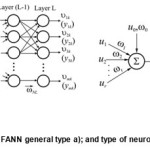
An artificial neuron, as per Mc Cullock & Pitts has limited ability in neuro-processing22. Having in minds the aforesaid complex structures are created in order to exert improved performances 23,24. Further on a focus will be paid onto ANN multi-layers feed-forward (FANN) and real-time recurrent neurel networks (RTRNN); (Fig. 1 & Fig. 2). Complex structures of FANN type shown in Fig. 1 having such
properties which enable successful training under supervising by using BPE21. It is worthwhile to point-out that almost all ANN can be transformed into FANN (BPE Throught Time (BPETT))25,26. What give enough reasons to start our further presentation with this type of ANN i.e. the FANN.
SDS Method in ANN Training
Throughout of FANN supervised training process an intention is to minimize an error at the network output excited by training pair:
esk(L) = ysk (t) – ysk (L) , …(1)
according to the cost function:
Qk = 1/2[Σ(esk (L) ]2 , … (2)
by iteration procedure:
ωv+1 = ωv + Δ ωv
where are: v -step of iteration; s=1,2,3,….,m; k= 1,2,3…..,K; K is number of training pairs pk = (usk, ysk(L)) in a set P; pk ∈ P, L is the layer on the end of FANN.
Back Propagation Error (BPE) uses iterative procedure :
∆ωij (l) = – α ∂Qk/∂ωij(l) ; 0<α≤1, …(3)
where are:
∂Qk/∂ωij(l) = [∂Qk/∂netj(l) ][ ∂netj(l)/∂ωij(l) ];
∂netj(l)/∂ωij(l)=υj(l-1); ∂Qk/∂netj(l)=δj(l); …(4)
i, j are indexes at two neurons at neighbouring layers l-1 and l. The motion δj(l) is important variable in optimisation process of BPE for FANN in back propagation stage after final completed forward step where succesive feeding of input out of set of training pairs21 SDS iterative procedures are performed in steps of random vectors varying for intire FANN network is:
∆ωv = α ort ξv , ΔQv<0 …(5)
i.e. as per layers l for ν successful step of iteration27;
∆ωij,v (l) = α ζij,v (l) …(6)
where are: l = 1,2,3,…,L ; i = 1,2,3,…N(l-1); j = 1,2,3,…,N(l)j ; l –layers FANN, i andj are neurons indexes of two adjacent layers, with total neuron number Ni(l-1) and Nj(l) ; ξ is random vector the same dimension as vector ω; 0< α ≤ 1; ν=1,2,3,…,Nε, where Nε is the final step of search; ζij,v(l) are the components of ortξv=ζv , |ζv |=1.
It has been previously mentioned that MN-SDS algorithm was created and suggested by the author27. Its basic version is defined by:
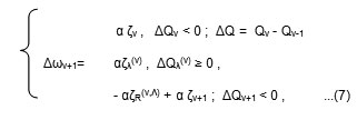
where: ζv = ort ξv ; ζv– is refered to v step of iterration, ∆Qv – increment of cost function Q in ν effective iteration step; ζR(ν,Λ) – is resultant of all failed steps ζλ(ν) , ∆Qλ(v) – increment of Q for failed steps λ, λ=1,2,3,…,Λ; ζv+1 is first step with ΔQv+1<0 after λ=Λ ; for ξ and ζ to apply the relation |ξ|≤1, |ζ|=1.
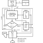
The using ortξ=ζ is nessesary for the improvement stability of process training. Minimum of a cost function Q is obtained in forward stage for particular choice of SDS algorithm. SDS does not require both nither differentiability and continuity of the activation function. SDS is rather more convinient when it is implemented jointly with simulation models during optimisation i.e. training process. For more complex ANN processes (number of dimension more the ten) almost all SDS algorithms exert better convergence performance compared to BPE methods5. The Fig. 3 shows diagram of MN-SDS numerical procedure.
Design Problems-ANN Synthesis
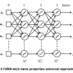
The synthesis problem of an ANN is rather complex one. On the other hand the said problem is not always formalised. Apart of intentions of various researchers to reach an answer mostly partial solutions have been offered for some specific ANN architetures. Somehow the experience of designers has crucial role in an ANN architeture choice related to neurel networks. In this chapter a simplified instruction for FANN choice are presented having under certain anticipations sourcing from theory of universal aproximator16-20. In Fig. 4 one form of universal approximator (UA) is presented.
If we, for a network with r inputs and m outputs assume number of neurons layerwise, than there are Nω interlinks between neurons in that network and Nϴ bias. A simplified assessment of required thraining samples based on theoretic results for UA18,20 is as follows:
Np = 10 (Nω + Nϴ). …(8)
where is: Np presents number of training samples in a set P required to have network generalization yield more then 90%, under constrains:
(r + Nvh ) ≫ m and C = Nω/m, …(9)
Nνh is a number of hiden neurons, C is a network capacity. It is not ease to satisfy condition for set of training samples. Mostly number of samples Np is not always enough. If there is a limit for samples number than is decrease i.e. unless relations given in (8) & (9) are settled. It is not expected to have neither unique & optimal solution since there is no limit for distribution of hiden neurons. Relation (9) indicate that there is no unique solution. It is not to be assumed as defficiency since there is enough space for optional solution in FANN architecture. For some other type of networks there is no an appropriate guideline as previously indicated.
An Application of Simulation Models in ANN Training
An application of simulation methods with iterative algoritms enables avoiding of mass calculation specifically when a network architecture is slightly complex. Simulation models are more convinient whenever real-time processes are in question. One of most complex ANN dynamic training methods incorporate so called simulated annealing process28. The simulated annealing process is rather combinatorial complex method, but also rather useful in ANN synthesis. However, presented simulation approach here is conceptualy connected with the theory of processes control. Presentation ANN over graf oriented form is the most appropriate to translate in the simulation model.
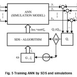
From the conceptual point of view an application of simulation models with SDS algorithms is shown in the Fig. 5. In the Fig. 5 G1 is random numbers generator, G2 is input signals generator, G3 is output of training pairs signal generator, Q is a block of cost function. The decision block DB for an iteration step–stop is not necessary to be positioned as indicated in the Fig. 5. An iteration steps whenever the condition Qv ≤ QNε atν=Nϵ i.e. min Q has been achieved.
In the Fig. 5 all elements of FANN network are replaced by appropriate components of simulation model. The reason to choose of MATLAB SIMULINK is facilitation of creation of simulation models both linear or non-linear functioning in real time. In addition to the aforesaid strong graphic environment and programming options for complex attempts29.
Examples
Example 1
Multy-layers FANN capable to reproduce the true table XOR circit.
An artificial neuron of a basic definition i.e. perceptron can not „recognize” XOR logic circuit. The previously said has a historical meaning30. If someone had used SDS algorithms than the neuro-science would not have stagnated almost 20 years.
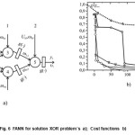
The two layers perseptrons as per the Fig 6.a) with the two neurons in hidden layer and the output neuron gives FANN capable to reproduce the true table XOR. In order to point out some advantages of MN-SDS let us the hidden neurons have the activation function as
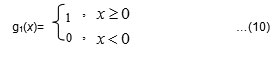
A direct implementation of BPE is not possible since g1(x) is not differenciable. The BPE implementation is possible if the function g1(x) is aproximated by the logistic function:
g2(x)= 1/(1+exp(-cx)); c ≥10 . …(11)
Available training pairs to be used in training process give the true table of XOR:
{Pk(u1,k, u2,k,}→[ P1(0,0,0), P2(0,1,1), P3(1,0,1),P4(1,1,0)]. …(12)
{ P´k(u‘1,k, u‘2,k ´)}→[P´1(-1,-1,-1),
P´2(-1,1;1), P´3(1,-1;1),P´4(1,1;-1)] . …(13)
where is k=1,2,3,4.
 
The stohastic search algorithm MN-SDS is aplayed to training ANN on Fig.6 a) over the series training pairs (13). For some variables in the Fig 6.a) a fixed values will be adopted.
U01=U02=0; U03=U04=U05= -1; ω01=ω02 =0 .
Further on number of variable parameters (n) for ANN in the Fig 6.a) is n=9. The random numbers vector ξ would have the same dimension. Its components would have indexes of certain weights as per the Fig 6.a).
So, the random vector ξ=( ξ1, ξ2,… …ξ9)T ; |ξq |≤1; q=1,2,…n; n=9.
The searching starts with an initial random choice ξ0 = ω0 :
ω0 = (0.873, 0.784, 0.953, 0.598, 1.013, 0.550, 0.740, 0.191, 0.573 )T.
Final values of components random vector after Nε ≥ 350 iteration with SDS algorithm i.e. MN-SDS for epoch i.e.for complete training set P are:
ωNε =(0.999, 0.997, 0.995, 0.998, 1.503, 0.990, 0.511, -1.982, 0.982 )T,
So, final values weights for ANN from the Fig 6.a) after arrounding are:
ωNε = (1, 1, 1, 1, 1.50, 1, 0.50, – 2, 1 )T, i.e.
ω13 =1, ω14 =1 ω23 =1, ω24 =1, ω03 =1.50,
ω04 =1, ω05 =0.50, ω35 = -2, ω45 =1. …(14)
The achieved relative error is less than 2%.
By using sequence of training pairs {P´k(u‘1,k, u‘2,k ´)} a better convergence is achieved during training process.
The trend of the cost functions behavior during the training process for each sample individually is shown in the Fig 6. b). In the same figure the cost function behavior is shown by use of BPE method for one single sample tp(1,1,-1). The trend of cost function for wholl epoch is similer. The optimization process i.e. training in that case is completed after N’ε ≥ 600 iteration.
Example 2
An intelligent monitoring of technological processes
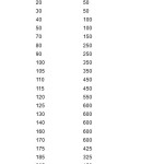
This example considers typical process related to numerous metallurgical & chemical technologies. Namely, it considers initial stages of tempering of agregates into rated production state and monitoring of situation when the agregate is down of regular operation as well. This case is related to tempering process of fluo reactors (FR) and smelters of metal raw materials. The tempering is usually recorded and measured data presented in the Table-127. Data from the Table-1 can be used to create regresion model.
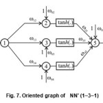
Instead of statistic methods it is possible to achieve over neuro models by using of so called universal approximator. Namely, it consider creation of three layer network with one input and one output. Since it contains complex interrelation it is advisable to start with the following architecture: 10 neurons (with linear activation function), 10 neurons in hidden layer (with non-linear activation function) and a neuron at output (with linear activation function). The aforesaid can be presented in the scheme NN10=(1-10-10-1). The first neuron at input operates as a demultiplexor. Since universal aproximator has the structure of FANN network that it is rather ease to get overall number of weights Nω =120 and overall number of thresholds Nϴ= 21. If we refer to relations (9) & (10) for generalization more then 90% it is necessary Np= 1410 training samples what is more that contained in the Table-1 That is the reason to reduce number of neurons as per scheme NN5= (1-5-5-1). For the previous architecture the number of training samples is 460. Consequently next reduction bring to NN2=(1-2-2-1) claiming to have some 130 training samples not available in the Table-1. In order to overcome this problem and realize the ANN model additional training samples at each 2min (with supposing the tempereture in FR until the next measurement does not change or with linear incrising) are necessary what would provide some 125; we can say almost 130 samples. Having in minds conditions from (8) and (9) the structure NN’=(1-3-1) could fit the case as shown in the Fig. 7. If for a nonlinearity activation function is used tanh(x), the final structure of ANN can be discribe with expression:
T(t)=ω25tanh(ω12t+ω02)+ω35tanh(ω13t+ω03)+ ω45tanh(ω14+ω04)+ω05 … (15)
By applying MN-SDS algorithm unknown parameters can be determined-weights ANN; in this case ther are ten:
ξ =( ξ1, ξ2, ξ3, ………., ξq)T,
|ξq|≤1, q=1,2,…n, n=10.
By random selection is determined the start values of weights:
ξ0 = ω0 = [0.1576, 0.9572, 0.4218, 0.8003, 0.7922, 0.9706, 0.9706, 0.4854, 0.1419, 0.9157]T. … (16)
After copmletition of the process optimization i.e. training for a whole epoch, the vector weights is:
ωNε = [ 1.705, 3.847, 11.61, 3.159, -3.597, 0.731, -1.670, -7.021, -13.23, 02939] …(17)
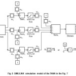
In the FIG. 8 it is presented a simulation model of the FANN on the Fig. 7. In conjunction with MN- SDS algorithm it can perform the training process. For discreet input values (independent of time) from the set of training sessions pairs mathematical procedure is relatively simple.
Example 3:
Training recurrent neural networks with time-varying
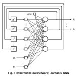
The aim of this example is that on conceptual level through the fully connected RNN in the Fig.2 (Jordan’s RNN), show that the use the coupling simulation model of network and SDS algorithms (according to the scheme on the Fig.5), formally is identical in procedures as in the case of training FANN. This approach to training is numerically simpler then numerical-analytical methods that use gradient of a cost function.
If inputs in RNN are time variable with duration T, network will posses dynamic behavior. This RNN is colled Real-Time RNN i.e. RTRNN31. Preform of input signals in discret form gives a series samples with τ repeat period; τ of sampling should be in accordance with the sampling theorem.
For discretized inputs may be indicated signals in RTRNN by:
- ui (n) – extern inputs,
- uj(n) – inputs of feedback link in network,
- xj(n) – interaction potencial for j neuron,
- yj(n+1)=gj(xj(n)) – extern actual outputs of certain neurons ;with out stimulus in time interval [n,n+1].
The error between the current value yj(n) and the desired value yj(d)(n) of actual output is
ej(n)= yj(n) – yj(d)(n) …(18)
The cost function Q is defined for one sample and all samples in the time interval T:
Q(n)= 1/2 [ej2(n)] …(19)
and
Qtot = Σ Q(n). …(20)
Analitical-numerical methods often for a step in procedure of optimization i.e. training use gradient of Q:
∆ω = – η ∇wQtot ; …(21)
where ∇wQtot is the gradient of Qtot ,
0 < η ≤ 1 ,
where: W – is a matrix of parameters i.e weights; η -is coefficient of a promptness learnings.
In SDS i.e. MN-SDS algorithm an iteration step is defined by (5) i.e.:
∆ω = α ortξ; ort ξ=ζ , |ξ| ≤1, |ζ| =1 …(22)
0 < α ≤ 1, α – is coefficient of a promptness learning’s.
Training of RTRNN based on the application of the MN-SDS and the simulation model of the same network (according to the Fig.5) is far simple and less subject to the phenomenom of unstable states than the case in analytical-numerical methods32.
The RTRNN type given on Fig.2 has significant performances. Their implementation is effective when it comes to projects predictionat non-stationary processes and phenomena33. In such cases training procedures are performed in the parameter space dimension of over 100.
Let us mention some numerous referring to the case when RTRNN on the Fig.2 reduced structure according to the following: the number of processing neurons is N=4, the number of line inputs is R=2 and the number of outputs is M=2. After the previous reducing the RNN on Fig.2, the new networks has:
N2+ NR = 42 + 4×2 = 24 interface link,
N2+NR+N=42+4×2+4=28 parameters (weights) to be determined in the process of training.
So, the random vector for applaying SDS is the same dimensions. With this level of dimensions SDS methods are more effective than BPE method ANN training.
The simulation model of reducing RTRNN is somewhat more complex than the model on Fig. 8. For RTRNN simulation it is need the SIMULINK with part for real-time processing.
In the case of optimization i.e. training a RTRNN shoud be taken appropriate scaling times T and τ due to the relationship, to the time required for computing the optimization cycles.
Discusion
Synthesis of an ANN is simply linked to its designing. Somehow the problem of synthesis formalization is a still open issue. Generally speaking the synthesis is well facilitated based on designer experiences and numerous available computer tools. This paper suggests an approach facilitating at least initial estimation of ANN structures. The said approach is based on a stochastic direct search method, implementation of the theory of universal approximation and application of simulation models.
An implementation of SDS algorithms in an ANN designing process deserves to mention that there are certain facilitation in optimization i.e. training of an FANN. A FANN optimization by implementation of SDS algorithm is performed in forward stage. That means quite reduced job to be expected compared to BPE method. The BPE method require multilayer FANN structure but if not, than it should be transformed into FANN. For SDS method it is easeness but transformation is not ever necessary, having in minds the presented approach in this paper. Attempts in other types of ANN into FANN transformation are useful since it enables use of results based on theory of universal approximation.
Strict explanation of an universal approximation is related to binary mapping of network input-output16. It could be said that it is intuitively adopted that the said theory is valid whenever mapping of continuous signals of network input-output. The author experiences indicate that the theory of universal approximator is rather correct. Simplification of some theoretical results facilitates to understand the paradigm of network ability to learn i.e. exert some inteligent behavior with more-or-less success. It is worthwhile to mention that training through optimization does not mean that network possess required level of ability to learn. Certain level of generalization provides conditions that network can recognize a samples not used in the training process( of the same population). In this approach to post-inspection training FANN through set of pairs of test not necessery. The theory of universal approximatlonr supports some relations in the FANN structure, mostly when hidden neurons with non-linear activation function are in question.
The choice of SIMULINK simulation port of MATLAB package is governed by practical reasons having in minds that it supports consideration both linear and non-linear objects including its vast graphical environment. The simulation is useful when recurrent neurel networks are considered specifically in real-time operation. By working with a RTRNN condition instability in networks may appear. combination of SDS & simulation methods is quite something new in an ANN designing process what enrich the designer experience.
The examples in this paper are two aims: a) comparison SDS and BPE (the first example), b) the others (two example) are chosen to illustrate the essence of this paper.
Conclusion
An application of stoshastic direct search method in design & training of artificial neuron networks offers a quite new approach having in minds numerical procedures efficiency vs known algorthms based on gradient features. It is well confirmed that for complex systems having unknown parameters more than ten, stochastic direct search shows remarkable advantages over gradient methods. In addition to the previous said SDS method is rather imune to presence of noice, ease iteration handling, adaptable against the problem nature and applicability to either systems with determined or stochastic mathematical description. This paper presents one new application of the MN-SDS algorithm, created by the author. The aforesaid integrates the properties of both non-linear algorithm and algorithm with accumulated information enabling to obtain self-learning ability.
The presented approach of design & training of neural networks is related so to the theory of universal aproximation. The said theory provides an insight into method of design and training of FANN, since it set up a conditions for hidden neurons having non-linear activation function in networks. Besides, the theory of univerzal approximation gives ration between number of interlinks vs the range of sinapses & scope of training samples. The simplicity presented in this paper provides rather accurate ratio and could be good orientation regarding starting assessment in a artifisial neural networks design.
The next feature of the presented approach is creation of straight interlink of stochastic direct search & simulation methods. The paper suggests implementation of SIMULINK method as software component of MATLAB package. The said package enables creation of linear & non-linear systems with lamp parameters with rich graphic environment. The SIMULINK provides options for presentation of neural networks in the form of oriented graph. The simulation model for the case of this form is easily acheieved regardless of the type of ANN. By carrying out the simulation process and MN-SDS for RTRNN unstable situation in network may take place. This last remark is a challenge for future researching. The obtained results out of numerical experiments related to the examples has been compared against BPE method and BPE through times. The comparison has shown the validity of results as well advantages of stochastic direct search. Numerical procedures has been supported by use of MATLAB R2014b, The Math Works Inc.
Acknowledgments
“For software Matlab in numerical experiments I am grateful to Mr. Milorad Pascas Research Assistant at the ICEF of Electrical Faculty University of Belgrade”.
References
- Rastrigin L. A., Stochastics Search Methods. In: Science Publishing, 1969; Moscow, Russia
- Dvorezky A., On Stochastic Approximation, In: Proc. III Berklly Symposium Math. Stat. and Probability, Vol.1, University of California Press, 1956; Berkeley, Calif, USA,
- Widrow B. and Hoff M.E., Adaptive switching circuits, IRE WESCON Convention Record, 1960; pp 96-104.
- Maquardt D.W., An algorithm for least squares estimation of non-linear parameters, J. Soc. Ind. Appl. Math, 1963; No 2, pp. 431-441,
CrossRef
- Rastrigin, L.A. Comparison of methods of gradient and stochastics search methods. In: Stochastics Search Methods, pp. 102-198. Sciece Publishing, 1968; Moscow, Russia
- Rastrigin L.A. and Rubinshtain L.S., Comparison of stochastic search and stochastic approximation method. In: The Theory and Application Stochastic Search Method, 1968; Zinatne, Latvia, pp. 149-156
- Zhiglavsky A.A., Theory of Global Random Search. Kluwer Academic, 1991; Boston.
- Baba N., Shomen T. and Sovaragi Y., A modified Convergence Theorem for a Random Optimization Method. Information Science, 1997; vol. 13, pp.159 – 166
CrossRef
- Spall J. C., Introduction to Stochastic Search and Optimization: Estimation, Simulation and Control Automation and Remote Control, 2003; vol. 26, pp. 224- 251.
CrossRef
- Nikolic K.P., An approach of random variables generation for an adaptive stochastic search. In: Proceeding ETRAN 96, Zlatibor, Serbia pp. 358-361.
- Nikolic K.P., An identification of complex industrial systems by stochastic search method. In: Proceeding ETAN 79; Maribor, Vol III pp 179-186.
- Nikolić K.P., An identification of non-linear objects of complex industrial systems. In: Proceeding ETRAN 98, Vrnjacka banja, Serbia, pp. 359-362.
- Nikolic K.P., Neural networks in complex control syst ems and stochastic search algorithms.In: Proceeding ETRAN 2009, Bukovicka banja, Serbia vol.3, pp. 170-173
- Nikolic K.P., Abramovic B., Neural networks synthesis by using of stochastic search methods. In: Proceeding ETRAN 2004, Cacak, 2004, Serbia pp. 115- .
- Nikolic K.P., Abramovic B. and Scepanovic I.: An approach to Synthesis and Analisys of Complex Neural Network. In: Proceeding of International Symposium NEUREL Belgrade, 2006
- Baum E.B., On the Capabilities of Multilayer Perceptrons, Journal of Complexity, 1988; vol.4., pp.193-215,
CrossRef
- Baum E.E. and Haussler D.: What Size Net Gives Valid Generalization?, Neural Computation, 1989; vol.1., pp.151-160
CrossRef
- Hornik K., Stinchomba M. and White H.: Universal Approximation of an Unknow Mapping and Its Devaritives Using Multilayer Feedforward Networks. Neural Networks, 1990; vol.3, pp.551-560,
CrossRef
- Hornik K., Approximation Capabilities of Multilayer Feedforward Networks. Neural Networks, 1991; vol.4. pp.251-257,
CrossRef
- Leshno M., Lin V.Y., Pinkus A. and Schockan S.: Multilayer Feedforward Networks With a Nonpolonomical Activation Function Can Approximat Any Function. Neural Networks, 1993; vol.6, pp. 861-867
CrossRef
- Rumelhart D.E., Hinton G.E. and Williams R.J.: Learning Representation by Back-propagation Errors. Nature, 1986; No 232, pp 533-536,
CrossRef
- McCulloch W.S. and Pitts W.: A logical Collums at Ideas Immanent in Neurons Activity. Bull. Mathematical Biophisics, 1943, vol.5, pp.115-133
CrossRef
- Grossberg S.: Nonlinear Neural Networks: Principles, Mechanisms and Architectures. Neural Networks, 1988; vol.1, pp 17-61,
CrossRef
- Nelson N.N. and Illingworth W.T.: A Practical Guide to Neural Nets. Addison-Wesley Publishing Company, Inc., 1991.
- P.J. Webros: Back-Propagation Time: What is does and how do it. Proc. of IEEE 78, 1960; pp.1950-
- Haykin S.: Back-Propagation Throught Time. In: Neural Networks(A Comprehensive Foundation), Macmillan College Publishing Company, 1994. New York, pp. 520-521
- Nikolic K.P.: Stochastic Search Algorithms for Identification, Optimization and Training of Artificial Neural Networks. International. Journal AANS, Hindawi, 2015;http://www.hindawi.com/journals/aans/2015/931379/
- Kirkpatrick S., Gellat C.D. and Vecchi M.P.: Optimization by Simulated Annealing. Science, 1983; vol.220 No. 4598, pp. 671-680,
CrossRef
- MATLAB 2014b, The MATH WORKS Inc, 2015
- Minsky M. and Pappert S.: Perceptrons. In: An Introduction to Computational Geometry, MIT Press, 1969; Cembridge, Mass.
- Haykin S.: Real-Time Recurrent Networks. In: Neural Networks (A Comprehensive Foundation), Macmillan College Publishing Company, 1994; New York, pp. 521-526
- Williams R.J. and Zipser D.:A learning algorithm for continually running fully recurrent neural networks. Neural Computation 1, 1989; pp. 270-280,
CrossRef
- Goh S. L., Popovic D., Tanaka T. and Mandic D.: Complex-valued neurel Network schemes for online processing of wind signal. In: Proceeding of International Symposium NEUREL, 2004; Belgrade, pp. 249-253

This work is licensed under a Creative Commons Attribution 4.0 International License.