Survey on Discriminative Least Squares Regression and its application.
INTRODUCTION
Least Squares Regression (LSR) is a widely-used statistical analysis technique. It has been adapted to many real-world situations. LSR earns its place as a fundamental tool due to its effectiveness for data analysis as well as its completeness in statistics theory. Many variants have been developed, including weighted LSR [1], partial LSR [2], and other extensions (for example, ridge regression [3]). In addition, the utility of LSR has been demonstrated in many machine learning problems, such as discriminative learning, manifold learning, clustering, semi-supervised learning, multitask learning, multiview learning, multilabel classification, and so on. The scope of this paper is to demonstrate all the application area of Least Squares Regression method in brief.
The method of least squares is a standard approach to the approximate solution of over determined systems, i.e., sets of equations in which there are more equations than unknowns. “Least squares” means that the overall solution minimizes the sum of the squares of the errors made in the results of every single equation. The most important application is in data fitting. The best fit in the least-squares sense minimizes the sum of squared residuals, a residual being the difference between an observed value and the fitted value provided by a model. When the problem has substantial uncertainties in the independent variable (the ‘x’ variable), then simple regression and least squares methods have problems; in such cases, the methodology required for fitting errors-in-variables models may be considered instead of that for least squares. Least squares problems fall into two categories: linear or ordinary least squares and non-linear least squares, depending on whether or not the residuals are linear in all unknowns. The linear least-squares problem occurs in statistical regression analysis; it has a closed-form solution. A closed-form solution (or closed-form expression) is any formula that can be evaluated in a finite number of standard operations. The non-linear problem has no closed-form solution and is usually solved by iterative refinement; at each iteration the system is approximated by a linear one, and thus the core calculation is similar in both cases.
Linear regression was the first type of regression analysis to be strictly studied. Given a data set {xi }ni=1 ϵRm and adestination set {yi}i=1Rc, where yiis the image vector of xi , the popularly-used regularization for linear regression can be addressed as an optimization problem
Formula1
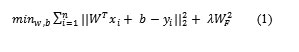
Where W ϵRm×c and b ϵRcare to be estimated and λ is a regularization parameter, || · ||2 denotes the L2 norm, and || · ||Fstands for the Frobenius norm of matrix.
In data analysis, (1) is often applied to data fitting where each yiis a continuous observation. When it is employed for data classification, yiis manually assigned as “+1/−1” for two-class problems or a class label vector for multiclass problems. For classification tasks, it is desired that, geometrically, the distances between data points in different classes are as large as possible after they are transformed. The motivation behind this criterion is very similar to those used for distance measure learning [4], [5].
INTRODUCTOIN OF REGRESSION ANALYSIS
In statistics, regression analysis is a statistical process for estimating the relationships among variables. It includes many techniques for modeling and analyzing several variables, when the focus is on the relationship between a dependent variable and one or more independent variables. More specifically, regression analysis helps one understand how the typical value of the dependent variable (or ‘Criterion Variable’) changes when any one of the independent variables is varied, while the other independent variables are held fixed. Most commonly, regression analysis estimates the conditional expectation of the dependent variable given the independent variables – that is, the average value of the dependent variable when the independent variables are fixed. Less commonly, the focus is on a quantile, or other location parameter of the conditional distribution of the dependent variable given the independent variables. In all cases, the estimation target is a function of the independent variables called the regression function. In regression analysis, it is also of interest to characterize the variation of the dependent variable around the regression function, which can be described by a probability distribution.
Regression analysis is widely used for prediction and forecasting, where its use has substantial overlap with the field of machine learning. Regression analysis is also used to understand which among the independent variables are related to the dependent variable, and to explore the forms of these relationships.
Regression models involve the following variables
The unknown parameters, denoted as β, which may represent a scalar or a vector.
The independent variables X.
The dependent variable, Y.
A regression model relates Y to a function of X and β.
Y ≈ f (X, β)
There are many types of Regression
There are many types of Regression
1. Simple Regression – fits linear and nonlinear models with one predictor. Includes both least squares and resistant methods.
- Box-Cox Transformations – fits a linear model with one predictor, where the Y variable is transformed to achieve approximate normality.
- Polynomial Regression – fits a polynomial model with one predictor.
- Calibration Models – fits a linear model with one predictor and then solves for X given Y.
- Multiple Regressions – fits linear models with two or more predictors. Includes an option for forward or backward stepwise regression and a Box-Cox or Cochrane-Orcutt transformation.
- Comparison of Regression Lines – fits regression lines for one predictor at each level of a second predictor. Tests for significant differences between the intercepts and slopes.
- Regression Model Selection – fits all possible regression models for multiple predictor variables and ranks the models by the adjusted R-squared or Mallows’ Cp statistic.
- Ridge Regression – fits a multiple regression model using a method designed to handle correlated predictor variables
- Nonlinear Regression– fits a user-specified model involving one or more predictors.
- Partial Least Squares – fits a multiple regression model using a method that allows more predictors than observations. Out of these models some of them are used for different machine learning problems such as multiclass classification, feature selection, depth estimation of 2d faces images and etc.
Applications of Least Square Regression
Application in Multiclass Classification problem
Given ntraining samples {(xi , yi)}ni=1 falling into c (≥ 2)classes, where xi is a data point in Rmand yiϵ {1, 2, . . . , c} is the class label of xi , our goal is to develop a LSR framework such that the distances between classes are as large as possible. One way to achieve our goal is to apply Leski’s twoclass LSR model [6] with the one-versus-rest training rule. This approach yields n independent subproblems where the subproblems have to be solved subsequently one by one. Here, we will develop a unique compact model for multiclass cases. Note that an arbitrary set of c independent vectors in Rcis capable of identifying c classes uniquely. Thus, we can take 0−1 class label vectors as the regression targets for multiclass classification. That is, for the j th class, j = 1, 2, . . . , c, we define f j = [0, . . . , 0, 1, 0, . . . , 0] T ϵ Rc with only the jth element equal to one [in other words, this is actually achieved in way of dummy (or unary) encoding where the 1 is the dummy]. Now our goal is to learn a linear function
Y = WT* x +T…………………(2)
such that for n training samples we have
fyi ≈ WT* x1 + t, i = 1,2,……..,n……………..(3)
whereW is a transformation matrix in Rm×cand t is a translation vector in Rc.
We see in the j th column in Y, only the elements corresponding to the data in the j th class are equal to one and all the remaining elements are zero. Thus, each column vector of Y actually stipulates a type of binary regression with target “+1” for the j th class and target “0” for the remaining classes. Although it is impossible for us to write out similar constraints used in two-class cases [6] with 0/1 outputs, we can drag these binary outputs far away along two opposite directions. That is, with a positive slack variable εi, we hope the output will become 1 + εifor the sample grouped into “1” and −εifor the sample grouped into “0.” In this way, the distance between two data points from different classes will be enlarged. This gears to the general criterion of enlarging the margin between classes for regression [7], [8].
After the regularized LSR framework, we can obtain a learning model as follows:
Formula 4
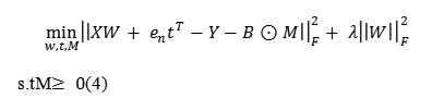
whereλ is a positive regularization parameter.
With our formulation, we see the c subproblems are grouped together to share a unique learning model. This will yield two advantages. One is that, even with the similar one-versus-rest training rule, we only need to solve them once for multiclass cases. Another advantage is that the model has a compact form, which can be further refined in order to implement feature selection based on sparse representation.
Application in Feature Selection
Suppose we are given n training samples {(xi, yi)}ni=1, which belong to c (≥2)classes. Here, xi ϵRm is a data point and yiϵ {1, 2 . . .c} is its class label. Our goal is to select d features from the original m features for classification. Straightforwardly, the task is to find a 0−1 selection matrix W ϵ {0, 1}m×dsuch that ˜x = WT x (ϵRd)is a sub-vector of x, where each row and each column in W has only one component equal to 1. Directly finding such a 0−1 selection matrix is proven to be a NP hard problem [42]. A commonly used way is to consider the feature selection problem by taking W as a transformation matrix. If some rows of W were equal to zero, the data dimensions that correspond to these rows could be removed, i.e., a selection of dimensions could be performed. We can formalize this as follows. Let Wibe the ith row of W. Then, a new vector w. , which collects the L2 norms of the row vectors of W, can be constructed as
Formula5
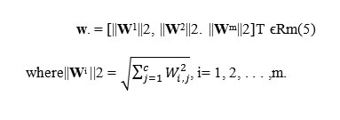
seethat constructing d nonzero rows in W is just equivalent to forcing the number of nonzero entities in w. equal to d
|| w. || 0 = d ….(6)
Unfortunately, directly solving the problem with constraints in L0 norm is also a NP hard problem. Alternatively, weconsider approximating L0 norm with L1 norm [43], [44] and use the following L2,1 norm of matrix W to develop thelearning model for feature selection
Formula7
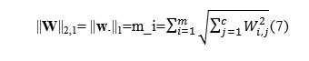
Now (7) can be extended for feature selection as follows:
Formula8
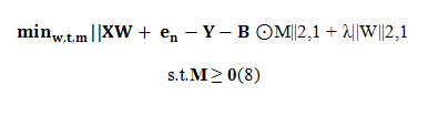
Where λ is a positive tradeoff parameter.Note that L2,1 is a norm. Thus, || · ||2, 1 is a convex function.Additionally, the constraint M ≥ 0 is also convex. Then, (8) is convex and has therefore only one global minimum [9].
Application in Cross Pose Face Recognition
Pose variation is one of the challenging factors for face recognition. In this paper, we present brief review on novel cross-pose face recognition method named as Regularized Latent Least Square Regression (RLLSR). The basic assumption is that the images captured under different poses of one person can be viewed as pose-specific transforms of a single ideal object. We treat the observed images as regressor, the ideal object as response, and then formulate this assumption in the least square regression framework, so as to learn the multiple pose-specific transforms. Specifically, we incorporate some prior knowledge as two regularization terms into the least square approach: 1) the smoothness regularization, as the transforms for nearby poses should not differ too much; 2) the local consistency constraint, as the distribution of the latent ideal objects should preserve the geometric structure of the observed image space [10].
Formally, we assume the pose can be discretized into p different bins. Let {X_}, k=1,…, p denote a set of training images, where Xk = {xijk| i = 1, … , c, j = 1, … , nik} denotes the samples in pose k, xijk ϵ Rd is the jth image of individual ifrom pose k in d dimensions, nik is the number of images for individual i under pose k, and c is the number of individuals.
Regularized Latent Least Square Regression is to deal with the cross pose face recognition problem. We assume that the images of one person captured under different poses could be mapped into a single ideal point in the latent pose-free space. The RLLSR framework provides such a way to formulate this assumption that it can integrate some regularization technology to improve the generalization performance efficiently. Comparative experiments indicated that the proposed method results in high accuracy and robustness for the cross pose face recognition problem.
Partial Least Squares for Dimension Reduction
Partial least squares based dimension reduction (PLSDR) is superior to handling very high dimensional problem such as gene expression data from DNA microarrays, but irrelevant features will introduce errors into the dimension reduction process and reduce the classification accuracy of learning machines. Here feature selection is applied to filter the data and an algorithm named PLS DRg is described by integrating PLSDR with gene selection, which can effectively improve classification accuracy of learning machines. Feature selection is performed by the indication of t-statistics scores on standardized probes. Experimental results on seven microarray data sets show that the proposed method PLS DRg is effective and reliable to improve the generalization performance of classifiers.
PLS is a class of techniques for modeling relations between blocks of observed features by means of latent features. The underlying assumption of PLS is that the observed data is generated by a system or process which is driven by a small number of latent (not directly observed or measured) features. Therefore, PLS aims at finding uncorrelated linear transformations (latent components) of the original predictor features which have high covariance with the response features. Based on these latent components, PLS predicts response features y, the task of regression, and reconstruct original matrix X, the task of data modeling, at the same time.
Partial Least Squares based Dimension Reduction (PLSDR) is a widely used method in bioinformatics and related fields. Whether a preliminarily gene selection would be applied before PLSDR is an interesting problem, which often was neglected. In this paper, we examined the influence of preliminarily gene selection by the t-statistic gene ranking method to PLSDR. We found the effect of gene selection greatly rely on data sets and classifiers, furthermore, simply selecting some top ranking genes is not a good choice for the application of PLSDR. Based on the notion that irrelevant genes are always not useful for modeling, we proposed an efficient and effective gene elimination method by the indication of t-statistic scores of random features, which improves the prediction accuracy of learning machines for PLSDR.
Text Classification Based on Partial Least Square Analysis
Latent Semantic Indexing (LSI) is a favorite feature extractionmethod used in text classification. Since when importantglobal features for all the classes can be determinedby LSI, important local features for small classes may be ignored,this leads to poor performance on these small classes.To solve this problem, a novel method based on Partial LeastSquare (PLS) analysis is proposed by integrating class informationinto the latent classification structure.
Text classification often suffers from the problem of highdimensionality of the texts. So above mention Partial Least Square based dimension reduction method is proposed for this problem domain also.
CONCLUSION
In this paper we brief Regression its application and all the important types of regression. Next we concentrate on least square Regression method and its application area. We conclude application of least square regression in multiclass classification, dimension reduction, face reorganization and etc. In all application area we brief a common steps and method to achieve high accuracy as an example we introduce concepts of ϵ dragging in multiclass classification to separate many classes efficiently.
REFRENCES
- T. Strutz, Data Fitting and Uncertainty: A Practical Introduction to Weighted Least Squares and Beyond. Wiesbaden, Germany: Vieweg, 2010.
- S. Wold, H. Ruhe, H. Wold, and W. Dunn, III, “The collinearity problem in linear regression, the partial least squares (PLS) approach to generalized inverse,” J. Sci. Stat. Comput., vol. 5, no. 3, pp. 735–743, 1984.
CrossRef
- N. Cristianini and J. Shawe-Taylor, An Introduction to Support Vector Machines and Other Kernel-Based Learning Methods. Cambridge, U.K.: Cambridge Univ. Press, 2000.
CrossRef
- K. Weinberger, J. Blitzer, and L. Saul, “Distance metric learning for large margin nearest neighbor classification,” in Advances in Neural Information Processing Systems 18. Cambridge, MA: MIT Press, 2006, pp. 1473–1480.
- P. Schneider, K. Bunte, H. Stiekema, B. Hammer, T. Villmann, and M. Biehl, “Regularization in matrix relevance learning,” IEEE Trans. Neural Netw., vol. 21, no. 5, pp. 831–840, May 2010.
CrossRef
- J. Leski, “Ho–Kashyap classifier with generalization control,” Pattern Recognit. Lett., vol. 24, no. 14, pp. 2281–2290, 2003.
CrossRef
- R. Duda, P. Hart, and D. Stork, Pattern Classification, 2nd ed. New York: Wiley, 2001.
- V. N. Vapnik, The Nature of Statistical Learning Theory, 2nd ed. NewYork: Springer-Verlag, 2000.
CrossRef
- Guo-Zheng Li; Xue-Qiang Zeng, Jack Y. Yang Mary Qu Yang, “Partial Least Squares Based Dimension Reduction with Gene Selection for Tumor Classification”.
- XinyuanCai, Chunheng Wang, Baihua Xiao, Xue Chen, Ji Zhou, “Regularized Latent Least Square Regression for Cross Pose Face Recognition”, Proceedings of the Twenty-Third International Joint Conference on Artificial Intelligence.

This work is licensed under a Creative Commons Attribution 4.0 International License.