Introduction
This paper addresses about, image inpainting or disocclusion and geometric image rearrangement. In image inpainting a special case is texture synthesis constrained by boundary matching with a seed texture. Here an image U is given where a few pixels or a whole region Ω is missing, we wish to recover the lacking information in the best possible way. To give a more precise statement to this problem, following principles should be kept in mind:
- The seed image should provide a guideline to the synthesis of the missing pixels. The result of inpainting should locally be visually close to parts of the known image.
- Besides the above principle, one might wish to consider a set of images, build a summarizing account of their properties, and use this as learned a posteriori knowledge.
- Our a prioriknowledge of some typical image properties (there are uniform regions, edges, texture, etc.) should provide other indications for the inpainting.
At yet a higher level, our understanding of the scene can give us hints at how to inpaint properly. As it is being enabled by recent computer vision technologies, nowadays geometric image rearrangement is becoming more popular. Recent retargeting methods propose effective resizing by examining image content and removing the regions that is not important. Typical carving algorithm helps to retargeting by iterative removal of narrow curves from the image, because of the iterative greedy algorithm no global optimization can be made, and something as simple as removing one of several similar objects is impossible. Since seam carving removes regions having low gradients, significant distortions occur when most image regions have many gradients.
Inpainting By Correspondence Maps
2.1. Formulation
We are given a known image (intensity function) u(α) defined on the pixels α € I/Ω for some Ω . Next step is to recover the unknown intensities u(Ω) for α € Ω. Our strategy is to define a correspondence map F : Ω – I/Ω and to paste the pixel values from the seed image as u(α) := u(F(α)).
The map F should be chosen so that the synthesized region looks as much as like parts of the seed image, its eight surrounding neighbours (Nα cannot contain α).Visual closeness of two pixel neighbourhoods Nα and Nβ can be measured using the usual Euclidean distance
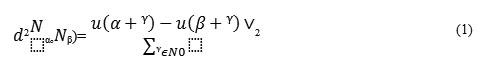
Where, N0 is for representing the neighbourhood of the origin. One can now define a global indicator of performance as
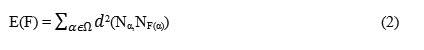
This is the objective to be minimized with respect to F. In other words, finding F amounts to filling Ω in the visually most faithful way by pixels of the seed image.
Our inpainting energy is at a much more elementary level than a regularization operations like Television, as per previous knowledge that it is defined with poor learned (a posteriori) knowledge or subjective (a priori) assumption on what the solution should look like. Minimizing E(F) is not really a model, it is hardly more than one possible low-level formulation of the inpainting problem. A set of pixel neighbourhoods built from a single texture or image sample does not qualify satisfactorily as a set of model parameters do.
2.2. Algorithm
The following algorithm is a descent for E(F). It is based on local minimizations at every unknown pixel and the information is grown from the border to the inside in multiple sweeps.
We follow the following steps:
- Random initialization of map F.
- Consider pixel α immediately near the border of Ω and inside Ω.
- Update F(Ω) by neighbourhood matching. This means finding a pixel β€ I/Ω 2 minimizer of d(Nα;Nβ) so that F(α) := β. Then assign u(α) := u(F(α)).
- Repeat 2 and 3 for all the pixels inside Ω and near the border. Then go to the next row which is not immediately adjacent, etc. until every pixel of Ω is visited.
- Sweep again the totality of Ω, i.e. repeat 2 through 4, until E(F) stagnates at a minimum value.
We can make the basic scheme faster and more efficient in a variety of different ways. The following are the improvements that can be implemented
Codebook Pruning
An exhaustive search is far from being necessary when looking for a good match among the seed pixels. To a subset of the seed pixels, one can restrict the search for a good neighbourhood match, e.g. not too far and randomly chosen from the current α. Codebook can be called as a set of neighbourhoods Nα, of the candidates α, this is codebook pruning.
More likely candidates
There are a few natural pixels to include in the set of candidates in the seed image. There are a few natural pixels, to include in the set of candidates in the image that is labelled as seed. They cannot be chosen randomly. If all the neighbours of a pixel α already have been inpainted, a good candidate for F(α) would be F(α-β)+β for β close to the origin. Thus larger regions of the known image can be likely to be copied in this way
Multiresolution
The construction of the correspondence map in a multiresolution way,successive refinements on embedded grids helps in. using an appropriate interpolation procedure,one can then recursively refine this guess at finer and finer resolutions Thus a much larger scale interaction can be occurred than the size of the neighbourhood.
Image Editing By Labelling Of Graph
In image rearrangement and retargeting, the relationship between an input image I(x, y) and an output image R(u, v) is defined by a shift-map M(u, v) = (tx, ty). Thereby the output pixel R(u, v) can be derived from the input pixel I(u + tx, v + ty). The optimal shift-map is defined as a graph labelling, here the nodes represent output pixel of image, and each output pixel can be labelled by a shift (tx, ty). The optimal shift-map M minimizes the following cost function:

Where, Ed is a term providing external requirements, and Es is a term defined over neighbouring pixels N. Here the α is a user defined weight balancing of the two terms and for all our examples, we are taking the value of α=1.
3.1. Single Pixel Data Term
To enter external constraints, the data term Ed is used. The different cases of pixel rearrangement, pixel removal, and pixel saliency are described in the following sub-sections.
3.1.1 Pixel Rearrangement
When an output pixel (u, v) should originate from location (x, y) ,all the shifts get a high energy except input image in which the appropriate shift gets only zero energy. This can be expressed in the following equation

3.1.2 Pixel Saliency and Removal
In the output image, specific pixels in the input image can be forced to appear or to disappear. If it is plotted on a graph,a saliency map S(x, y) will be very high for pixels to be removed, and very low for salient pixels which should not be removed. So for the same reason the data term Ed for an output pixel (u, v) with a shift-map (tx, ty) will be,

3.2. Smoothness Term for Pixel Pairs
If the shift maps of two neighboring locations are different, a shift-map discontinuity exists between two neighboring locations (u1, v1) and (u2, v2) in the output image R. it can be equated as below:

Also the smoothness term Es(M(p),M(q)) represents discontinuities in the shift-map by discontinuities added to the output image. In addition to it,the smoothness term Es(M) takes into account both color differences and gradient differences between corresponding spatial neighbors in the output image and in the input image to create good stitching. Both the color differences and gradient differences are used for smoothness for the better preservation of structure. Many of the theoretical guarantees of the alpha expansion algorithm are lost because of the use of non-metric distances. But nowadays, in practice we have found that good results are obtained and also can be found that better results can be obtained by squaring the difference than using absolute value, preferring many small stitches over one large jump.
4. Continuous Images and Image Composition
To minimize the total inpainting energy over F, we have to model the image U as a function from I ∩ R2 to R, and the correspondence map as a function F from Ω∩ R2 to I/Ω∩R2. It can be expressed as follows:

But the case of image composition can be different. Either a simple image or a set of images can be constrained in an input in the shift-map framework. The shift-map M(u, v) = (tx, ty, tind) in multiple input images, where tind is the index of the input image used for each pixel. Producing an image rearrangement involving multiple images (selective composition) are also possible now,as the label of each pixel consists of both shifting and source image selection. Misalignments between the input images can be tolerated by the shift-map. As various areas can move differently with respect to their location in the input, the resulting composite image can be a sophisticated combination of the input images.
5. Inpainting and Remarks on the Algorithm
Inpainting image regions can be done by using shift-map. An automated process completes the missing area from other image regions or from other images, after interactive marking of unwanted pixels. The unwanted pixels are given an infinitely high data term using shift-maps. The main function of the shift-map is that, it maps pixels inside the hole to other locations. The missing pixels are copied from their source location at the time where mapping is completed by performing graph cut optimization. Only a local consideration can be made in each step due to the reduction in the size of the hole of existing inpainting algorithm. Under shift-map approach, inpainting is treated as a global optimization and thus the entire content is considered at once. Without any user intervention, shift-map approach can make a good completion.
Shift-map can even be used for generalized inpainting. The peculiarity of generalized inpainting is that, all the pixel labels can be computed irrespective of the pixels in the neighborhood of the hole. It adds increased flexibility to reconstruct visually pleasing images when it is easier to synthesize other areas of the image. Inpainting will turn to an image rearrangement problem under the situation where some areas should not move and other areas should be removed, user constraints can be added.
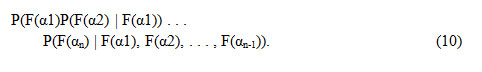
Now there is a need to clarify the deeper link between the formulation in terms of inpainting energy and the pixel-pasting-by-neighborhood-matching algorithm. Now let us a have a look to casual neighborhood. Here we are going to number the pixels of Ω in raster-scan order as α1, α2… α n. When pixel αi is visited we have to solve the following problem consisted in algorithm
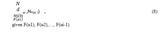
For notional convenience, we drop the seed image u on I/Ω which is also hidden in the constraints. There is another concept called `causality’ property of the neighborhood that the values of F(αi+1), . . . are not present in the condition. Maximization of the conditional probability can also be seen like this:
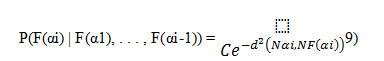
The constant C is an appropriate normalization constant. In fact, causality of neighborhood is a clever way to factorize it through Bayes’ rule as
Hence, the global `inpainting energy’ is therefore nothing but,
E(F) = -log P(F(α1), . . . , F(αn))
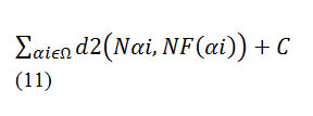
For some unimportant constant C.
Performing the successive neighborhood matching is much easier than obtaining the global minimum and is true regardless of the fact that the neighborhood is casual or not. Undoubtedly we can say that the very fast greedy procedure to reach a good point of low energy is nothing but successive minimization. Thus the success of algorithm can be understood in this way. Depending on the order in which pixels are taken, different values for the joint probability are given by the formal application of Bayes’ rule.
To consider the non-casual case, the right conditional probabilities are:

All the values of F for the pixels in Nα refers to the notation F(Nα). The distance ~ d is defined as:
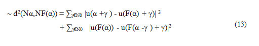
By using the new distance ~ d instead of d above, new algorithm can be modified. The main advantage of the new distance is that the global energy is decreasing at each step, which is not so in the case with d and also can be guaranteed to reach a local minimum. As usual, this reformation also have a drawback. As a result of this change, the algorithm becomes a pure descent and loses all its `creativity’ to find a good local minimum. By copy pasting pixels from a flat smooth region in the seed image, it would produce uniformly gray or colored regions. This is the reason for preserving the original d in our algorithm.
Conclusion
Through this paper, describes various geometric rearrangement problems computed as global optimization. This new framework is nothing but the shift-map which was discussed above. One of the main characteristic which distinguishes shift map from other geometric rearrangements is that the images generated by the shift map are natural looking. It also contain some of the desired properties as below:
- There are only minimal and intuitive user interaction and also no need for selecting the objects accurately.
- The global smoothness term minimizes the distortions which might be introduced by stitching.
- The geometric structure of the image is also preserved clearly.
- As we seen in all examples, large regions can be synthesized.
This paper has also dealt with inpainting. The low level inpainting solution helps in minimizing. There are some notion of visual closeness which is associated with the energy. In terms of similarity of neighbourhood, there exists a pixel in the seed image in good agreement for every synthesized pixel. If the correspondence map took the observer to a very distant pixel every time a step is taken in the missing region. Our expectation rather than isolated pixel is that large patches is to be pasted into that region reasonably and thus we can require the smoothness of the correspondence map.
The next important point is that, for texture synthesis, the algorithm is well suited; whereas sometimes it fails to reproduce geometrical features of the image. Inclusion of input image is worthwhile for the transformation of original input image like rotation, scaling etc. Moreover the algorithm will also help in controlling the effects of the shift map by the use of saliency map or by the performance of several algorithm steps.
References
- M. Ashikhmin. Synthesizing natural textures. In The proceedings of 2001 ACM Symposium on Interactive 3D Graphics,pages 217.226, March 2001.
CrossRef
- C. Ballester, M. Bertalmio, V. Caselles, G. Sapiro, and J. Verdera. “Filling-in by joint interpolation of vector fields and gray levels.”, IEEE Trans. on Image Processing, 10(8):1200.1211, August 2001
- M. Bertalmio, L. Vese, G. Sapiro, and S. Osher. Simultaneous structure and texture image inpainting. UCLA CAM Report 02-47, July 2002.
- P. Br´emaud. Markov Chains: Gibbs fields, Monte-Carlo simulation, and queues. Springer, 1999.
CrossRef
- T. F. Chan, S.-H. Kang, and J. Shen. Euler’s elastica and curvature-based image inpainting. SIAM J. Appl. Math, 63(2):564.592, 2002.
- A. Criminisi, P. P´erez, and K. Toyama. Object removal by exemplar-based inpainting. In CVPR’03, volume 2, pages 721–728, 2003.
CrossRef
- J. Hays and A. Efros. Scene completion using millions of photographs. CACM, 51(10):87–94, 2008.
CrossRef
- V. Kolmogorov and R. Zabih. What energy functions can be minimized via graph cuts? In ECCV’02, pages 65–81, 2002.
CrossRef
- N. Komodakis. Image completion using global optimization.In CVPR’06, pages 442–452, 2006.
CrossRef

This work is licensed under a Creative Commons Attribution 4.0 International License.