Introduction
XML documents have a tree structure called DOM. On the other hand, languages, which are used to respond queries, have a textual structure. Therefore, this structure conversion is necessary. In continuance, because of not requiring to be related to a special language, we define a structure called Tree Pattern Query. Fortunately, all query languages in XML are simply convertible to TPQ.
TPQ is a Tree Structure for XML queries. The tree nodes are composed of query tags and its mainscontain the linkages //, /, ? and *, so that for each element a and b with the linkage c, we can find a mane in TPQ that its nodes are a and b and its kind of mane, c.
Following on, we will explain the way to convert this XPath to TPQ with an example.
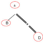
Example: Q1://A[./B]/*//D
In this query, A,B and D mean the tags we are looking for in the document. // means ( Ancestor – Descendant ) relation, / means ( Parent – Child ) relation and * is the name of the arbitrary tag. Now, TPQ can be depicted corresponding with the above query easily.
Now after being able to convert queries structures to the tree structure like the document, we can look for all tree models that match TPQ. For example if we want to perform the above queries on the below document, one of the attained models is < A2, B1, D1 >.
Reviewing the previous methods
Nested Loop Method
As stated in the previous part, a document is shown as a set of nodes and in the form of a tree. On the other hand, all query languages in XML require the match between query nodes and document. For example suppose we export the following query:
BOOK//title
It means we want all titles of the books. In this method, we firstly find all the books and then we test for each node if it has a child called title. This is the first method which is applied.
As it is clear, this method has many basic difficulties that we refer to two main cases which make it non-establishable for large documents:
In this method, a loop should be performed for each node. For example, if we want to perform the query, a/b//c/d, we will require 4 complex loops, so the time complexity of this method is O(n2), where n is the number of query nodes.
In this method, the number of the produced intermediate results is so much, and in addition to wasting time for processing these useless nodes, we will require a very large memory to hold these nodes.
Structural Join Method
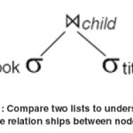
In this method, at first, all complex relations of the nodes are achieved. For example, the query, a//b/c//d is converted into the three relations, a//b, b/c and c//d; then each query is performed separately, and finally, the results are integrated altogether. We will explain the way of achieving one of the binary queries as follows. Note to the query, Book//Title. In this method, we will make two lists, for these two groups, one for the book and another for the title separately. Now, we compare all title nodes with all book nodes. We will return every pairs of nodes which have an Ancestor – Descendant relation between them as the response. This is called Join in database world.
This method has two general difficulty
- In this method, we have to divide the main query, which has a few responses into a large number of binary queries, which each one returns a large number of the responses.
- This method returns a large content of the intermediate results that a general content of the results will not be of the final result. Thus, producing and holding of these intermediate results make the response time to the main query longer.
Since this method breaks all queries to binary relations, we will need n-1 binary query and also m=(n-1)/2 integration for a query with n
member in the first step. So in general state, the time complexity of O(m(2+2(n-2))) for this query will be just in the first step. In later steps, the gained results is half on average. Since the first step of this method is the most time-taker step, we stated this step complexity as the method complexity.
Many of the studies on the above method have been done to increase efficiency and decrease time respond. For example, some papers have performed indexing two comparable lists, using the methods +B or +R. on the other hand, some methods compare the two lists as optimum, that means unrelated elements are not compared to a possible extent.
Staircase Method
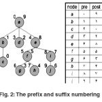
There is another familiar and useful method, that is Staircase Join. This method works as the previous method to some extent. In this method, the tree, firstly is surveyed in two forms of prefix and suffix. For example, below there is a piece of a tree with its numbering.
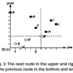
Now we write the tree with the new numbering to the two- dimensional space, so that the proper nodes are placed in each systemic node. For example, at the right and down side, Children and at the left and up side, Ancestor nodes of a node are placed. For instance, note to the situation of the node g in the tree and the diagram.
Now, we limit our seeking area to one of the four sides with this method. For example, in the previous query, Title seeking area was limited just to the children of a Book which were at the right and down side of this node. So, in the best state, the tome complexity of this method is 1/4 of the previous method complexity. Most of the methods such as [1] try to increase the efficiency of this method with loping the above method. In addition not to be optimum, all the stated methods have other problems such as replacement of the nodes situations or impossibility of updating, optimization, algebraic displaying and so on.
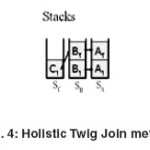
Holistic Twig Join
Another method which is in [15, 16, 17] has attained more acceptance rather than its previous methods; this method name is twig join Holistic. This method numbers the tree as an area like structural joint, then saves all the same nodes with each query element in separate stacks. At every moment, it tests if it can make a sample of TPQ. Two remarkable and different methods to find the relationship between stacks elements are Twig and Stack.
This method has this advantage rather than previous methods that there isn’t a requirement to analyze a query to a number of binary queries, so the number of intermediate results which are produced are much fewer. Since each list in this method is surveyed just once, time complexity of this method equals to O(Max(n1, n2, …, nm)). n means query nodes.
But one of the method problems rather than the later methods is to make all query nodes accessible in the real document. For example if we want to perform the query a/b/c, requirement to all sample of this node will be real. Thus we will encounter the problem of the high content of conceptual intermediate nodes (Figure 2.6).
But this method took many researchers’ attention, and a lot of studies were done for increasing its efficiency. For example, in [16], it tries to accelerate this method by indexing internal nodes in a B+Tree, or in [17], an index called XR_Tree was invented for this purpose. In [18], it’s been tried to decrease the number of required nodes by making changes on primitive algorithm. Today, this method is one of the useful ones, and even it could be said in some cases that it works better than its later methods, in special conditions.
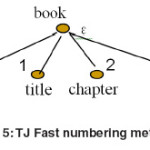
TJFast Method
All previous methods had to achieve all existent nodes in document for responding to queries. But in [56], by giving a method called TJFast, it proved that just by achieving query leaf nodes, it could get the response. For example, to respond the query Q1, we will just need to achieve Book and Title leaf nodes.
STUDENT//BOOK[TITLE=’XML’];
This method numbers the tree as decimal or Dewey encoding19,20, lets take a look at the encoding method at first. Using the encoding method, we will be able to produce a graphic called FST. This atamata can simply show the way of numbering the document. Using this atamata, encoding and decoding will be establishable. For example, by using of this atamata, it firstly encodes internal nodes, and then compares them to get the response. TJFast only compares query leaf nodes, so the number of accessible nodes in this method is much fewer than the similar one. For example, for a query of n branches with m members where n<<m, we will just need to test n members. As a result, the time complexity of this method could be written O(m). But on the other hand, the method has the following main problems:
In many cases, the time and content of FST is remarkable, and using it is uneconomic.
TJFast spends a lot of time to encode the nodes, and in a case, this causes the total time to be more than of the similar methods.
The Methods Based on Path Indexes
All the methods stated before are known as Containment join in XML world. This group of the methods applies an index called name index. The name indexes action is quick achieving to the elements with namesake tags. Consider the following query as an instance:
STUDENT//BOOK[TITLE=’XML’];
This index makes all Student, Book and Title nodes immediately available for algorithm for this query. For example, it keeps all the Book nodes in one array and processes them respectfully.
There is a main problem within all the above methods. This group of the methods regardless of the elements location, look for a way to binary compare of the nodes optimally; they try to get the query respond directly by these comparisons, while most of them attain no respond of the query.
The way that this group applies to respond queries is that at first, they compare the structural relation of (a – c or a – d) among queries with structural Summary, or in better words, they performs the query on SS firstly, then return Extend, the branches nodes which match with query as query respond. The primary algorithm of IT production for a two-branch query is as follows. This is a primary quasi code and it’s just for two-branch queries. The algorithm for complex queries is as follows.
Input: Q as TPQ
Output: IT as Index_Table
1: Let A and B the two leaves of Q
A and B are two query leaf node.
2: Let JP = Joint point between A and B
The connection point shows two-branch connection node.
3: Let AL = list of SS nodes match A branch
4: Let BL = list of SS nodes match B branch
A and B are identified by Extend nodes of the lists, AL and BL, respectfully. These nodes are the same found leaf nodes for each query branch.
5: for each an ∈ AL do
6: for each bn∈ BL do
7: for each JP1 in an , JP2inbn do
8: if an.Prefix(JP1) = bn.prefix(JP2) then
9: IT.addREC(an, bn, JP1.level))
10: end if
11: end for
12: end for
13: end for
The final results is made regarding the results table. Each record of this table guides the query processor to get a piece of the respond. The collection of these pieces produces the final result. Therefore, the final result is the collection of the returned results by each record.
The jumps over the nodes not participated in the final result
The nodes which are not participated in the final result are counted as usefulness conceptual nodes, and should be jumped over them. Note to the lines, 11 and 13 of the quasi code which has come for the final result production. These two lines are for the nodes group which haven’t had a successful corresponding action, and the pointer should goes on the next node. But what node is the next one?
The state Next in these two lines makes sequential processing among the elements. It means the elements are achieved by the pointer respectfully. But this node can’t have a successful correspondence since most of the nodes has a same prefix with their previous element, and if the previous element doesn’t have a successful correspondence.
We need to jump for the elements which don’t have a successful correspondence. The jump should be done over all the elements which have a same prefix to the connection point level.
Jump
if the node A is with the number a1/a2/…/aj/…/an and we want to have a jump in the level J, the next node will be B, if B is the smallest node which is larger than A and has a dissimilar prefix to the level J with the node A.
The Use of the Index Table on Indexed Leaves
As observed, we need an index that allows jumping from one node to another in a desirable level L. Here, we provide a primary multi list plot, and then complete level index plot for this kind of jumps. But before doing so, we consider two concepts of Jump and Level that are used a lot. Notice that the Extends of each group of SS, the query leaves in document, are indexed separately, because these nodes are considered as quasi code internals in the figure.
Multi list is a multiplet index for each level of ordered leaf nodes with level L, so that its highest level L-2 is assumed a root with Dewey of code1, and its lowest level will be L-1. Each list of ML with the level Li has the prefix of all the list nodes Li+1 to the level Li. Each node of ei in a list with the level ihas a pointer to the first leaf node beginning with ei.
One of the biggest problems of this method that makes it none-establishable is effluence in updating, deletion and interpolation. In the worst state, a deletion (interpolation) can enter the indexes of all levels.
Example: If we want to interpolate the node 1.1.4.1 to the leaves, we have to add 4.1 to the list of level 2 and 1.4.1 to the list of level 3.
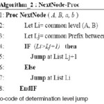
JUMP: The Jump quasi code in LBI is shown in the figure. Below, we explain its lines with example.
If it’s required to jump in the L2, from the current node N in the level L1 of index, if L1<L2, we should do a deep survey toward the level L (Line 2 and 3).
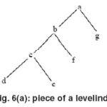
Example
The following figure shows a piece of a LBI. The root of the tree a is the level 1. The current node b is with the level 2; and we want to have a jump in the level 4. The order of the next accessible nodes is as c, d, e, …
If L2<L1, the first homo-ancestor node is next to the ancestor N in the level L2 (The lines 4 and 5).
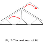
Considering the above diagrams, LBI index doesn’t act similarly, and its usage is not equal in all cases. But considering the above diagrams, the best and the worst states of the appliance could be stated as follows:
The best form of the tree:When Dewey number of internal nodes is near one another, (for example, the numbers such as 1/2/2/1/2, 1/2/2/1/1, 1/2/2/2/1, 1/2/2/2/3) or in other words, the nodes have similar prefixes to the lower levels of their Dewey, figure LBI will be like the figure below. In levelindexthis state, it is said that the fatness of the tree has occurred in the lower levels that makes the nodes content in LBI to be more in the lower level, so when we evaluate a node in upper levels, if it has a successful correspondence process, we have found many respond nodes just by one comparing; and if it has an unsuccessful correspondence process, we will jump over many sets of useless nodes.
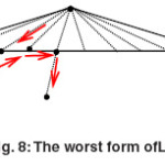
The worst form of the tree: when the interval among internal nodes in the real tree is high, it makes the nodes to have shorter quasi prefixes (for instance Dewey numbers such as 1/1/2/3/4 and 1/2/4/2), so the nodes gathering will be happened in higher levels of L1, and it’s said that the fatness of the tree exists in the head and the waist of the tree. Notice the following figure as an instance. In this state, our jumps are so little, so we may have more I/Q rather than the state that our internals are read respectfully.
For example, if you look at the red flashes, you will see that 5 node is read (that each can produce one I/Q), and jumping is just over one node (the blue node).
References
- Ramanan P. “Holistic Join for Generalized Tree Patterns “ , Information Systems, 32(7): 1018-1036 (2010). ELSEVIER.
CrossRef
- Kaushik. R., Bohannon. P., Naughton J. and Korth. H, Covering Indexes for Branching Path Queries, In Proc. 11rd SIGMOD Conference: 133 – 144 (2008)
- Kaushik. R., Krishnamurthy. R., Naughton. J., and Ramakrishnan. R. On the integration of structure indexes and inverted lists, In Proc SIGMOD Conference: 779 – 790 (2009)
- Goldman. R., Widom. J. DataGuides: “Enabling Query Formulation and Optimization in Semistructured Databases.”, In Proc. 23rd VLDB Conference: 436—445 (2011)
- Nestorov S., Ullman J., Wiener J., and Chawathe S., Representative Objects :” Concise Representations of Semi structured, Hierarchical Data “,In Proc. ICDE: 79-90 (1997)
- Chung, C., Min, J., Shim, K. Apex:” An adaptive path index for xml data.”, In Proc ACM Conference on Management of Data SIGMOD: 121 – 132 (2005)
- Cooper. B., Sample. N., Franklin. M., Hjaltason. G.,Shadmon. M. A Fast Index for Semistructed Data, In Proc. 14th VLDB conference: 341 -350 (2006).
- R. Kaushik, P. Shenoy, P. Bohannon, and E. Gudes.”Exploiting Local Similarity for Indexing Paths in Graph-Structured Data”. In IEEE/ICDE, pages 129-140, San Jose, California (2010).
- Al-Khalifa.S., Jagadish. H.V., Koudas.N., Patel. J.M., Srivastava. D., Wu. Y. Structural Joins:”A Primitive for Efficient XML Query Pattern Matching.”, In Proc. ICDE: 141-152 (2011)
- Chien. Et. “Efficient Structural Joins on Indexed XML “,In Proc. VLDB Conference (2011)
- Jiang.H.,Wang.W, Lu. H, and Xu Yu, J, anChin. B, XR-Tree: “Indexing XML Data forEfficient Structural Joins. “,In Proc. ICDE Conference :253-264 (2008)
- Mathis. C., Härder. T, Haustein. M. “Locking-Aware Structural Join Operators for XMLQuery Processing”, In Proc SIGMOD Conference: 467 – 478 (2008)
- Wu. Y., Patel. M. J. and Jagadish. H. V. “Structural join order selection for XML query optimization”, In Proc. VLDB Conference, (2012)
- Kaushik. R., Krishnamurthy. R., Naughton. J., and Ramakrishnan. R. On the integration of structure indexes and inverted lists, In Proc SIGMOD Conference: 779 – 790 (2009)
- E. Damiani, S. De Capitani di Vimercati, S. Paraboschi, and P. Samarati “A Fine-Grained Access Control System for XML Documents”. ACM TISSEC, 169-202, (2010).

This work is licensed under a Creative Commons Attribution 4.0 International License.