Different Methods for Statistical Face Representation - Review

T. Syed Akheel¹, S.A.K. Jilani² and K. Kanthamma²

¹P.V.K.K Institute of Technology, Anantapur (India).

²MITS Madanapalli (India).

ABSTRACT:

Face is an important biometric feature for personal identification. Human beings easily detect and identify faces in a scene but it is very challenging for an automated system to achieve such objectives. Hence there is need to have reliable identification method for interacting users .In this paper we discuss past research on biometric face feature extraction and recognition of static images. We will present implementation outline of these methods along with their comparative measures and result analysis.

KEYWORDS: Face recognition; Feature based methods; Fisher’s Linear Discriminant (FLD)

Copy the following to cite this article: Akheel T. S, Jilani S. A. K, Kanthamma K. Different Methods for Statistical Face Representation - Review. Orient. J. Comp. Sci. and Technol;4(1)

Copy the following to cite this URL: Akheel T. S, Jilani S. A. K, Kanthamma K. Different Methods for Statistical Face Representation - Review. Orient. J. Comp. Sci. and Technol;4(1). Available from: http://www.computerscijournal.org/?p=2354

Introduction

The developing of face recognition system is quite difficult because human faces is quite complex, multidimensional and corresponding on environment changes. For that reason the human machine recognition of human faces is a challenching problem due the changes in the face identity and variation between images of the same due to illumination, pose variations and some natural effects.The issues are how the features adopted to represent a face under environmental changes and how we classify a new face image based on the chosen representation.Computers that recognize human faces systems have been applied in many applications such as security system, mug shot matching and model-based video coding.

The eigenfaces is well known method for face recognition. Sirovich and Kirby¹had efficiently representing human faces using principle component analysis. M.A Turk and Alex P. Pentland² developed the near real-time eigenfaces systems for face recognition using eigenfaces and Euclidean distance.

Most effort in the literature have been focused mainly on developing feature extraction methods and employing powerful classifiers such as probabilistic hidden Markov models (HMMs) [4,36] neural networks (NNs)^3,5 and support vector machine (SVM)^4,37. The main trend in feature extraction has been representing the data in a lower dimensional space computed through a linear or non-linear transformation satisfying certain properties. Statistical techniques have been widely used for face recognition and in facial analysis to extract the abstract features of the face patterns. Principal component analysis (PCA)^1,7,8 and linear discriminant analysis (LDA)^3,7 are two main techniques used for data reduction and feature extraction in the appearance-based approaches. Eigen-faces and fisher-faces⁶ built based on these two techniques, have been proved to be very successful. LDA algorithm selects features that are most effective for class separability while PCA selects features important for class representation. A study in¹⁰ demonstrated that PCA might outperform LDA when the number of samples per class is small and in the case of training set with a large number of samples, the LDA still outperformthe PCA. Compared to the PCA method, the computation of the LDA is much higher [4] and PCA is less sensitive to different training data sets. However, simulations reported in [4] demonstrated an improved performance using the LDA method compared to the PCA approach. When dimensionality of face images is high, LDA is not applicable To resolve this problem we combine the PCA and LDA methods, by applying PCA to preprocessed face images, we get low dimensionality images which are ready for applying LDA. Finally to decrease the error rate in spite of Euclidean distance criteria this was used in [4]. A system is implemented using neural network to classify face images based on its computed LDA features.Kirby and Sirovich¹¹ showed that any particular face can be¹ economically represented along the eigenpictures coordinate space, and ² approximately reconstructed using just a small collection of eigenpictures and their corresponding projections (‘coefficients’).Turk and Pentland [12] applied PCA technique to face recognition, and proposed the well-known eigenfaces method. A recent major improvement on PCA is to directly manipulate on two-dimensional matrices (not one-dimensional vectors as in traditional PCA), e.g., two-dimensional PCA (2DPCA) [13], generalized low rank approximation of matrices [14], non-iterative generalized low rank approximation of matrices (NIGLRAM)¹⁵ and so on. The advantages of manipulating on two-dimensional matrices rather than one-dimensional vectors are [13]: (1) it is simpler and straightforward to use for image feature extraction; (12) it is better in terms of classification performance; and (13) it is computationally more efficient. Based on the viewpoint of minimizing reconstruction error, the above PCA-based methods [12,13–15] are unsupervised methods that do not take the class labels into consideration.Taking the class labels into consideration, LDA aims at projecting face samples to a subspace where the samples belonging to the same class are compact while those belonging to different classes are far away from each other. The major problem in applying LDA to face recognition is the so-called small sample size (SSS) problem (namely, the number of samples is far less than sample dimensionality), which leads to the singularities of the within-class and between-class scatter matrices. Recently, researchers have exerted great endeavor to deal with this problem. In [6,7], a PCA procedure was applied prior to the LDA procedure, which led to the well known PCA+LDA or Fisher faces method.In [7,8], samples were first projected to the null space of the within-class scatter matrix and then LDA was applied in this null space to yield the optimal (infinite) value of the Fisher’s linear discriminant criterion, which led to the so-called discriminant common vectors (DCV) method. In [19, 20], LDA was applied in the range space of the between-class scatter matrix to deal with the SSS problem, which led to the LDA via QR decomposition (LDA/QR) method. In [3] a general and efficient design approach using a radial basis function (RBF) neural classifier to cope with small training sets of high dimension, which is a problem frequently encountered in face recognition, is presented. In order to avoid over-fitting and reduce the computational burden, face features are first extracted by the principal component analysis (PCA) method. Then, the resulting features are further processed by the Fisher’s linear discriminant (FLD) technique to acquire lower-dimensional discriminant patterns. These DR methods have been proven to effectively lower the dimensionality of Face Image. Furthermore, in face recognition, PCA and LDA have become de-facto baseline approaches. However, despite of the achieved successes, these FR methods will inevitably lead to poor classification performance in case of great facial variations such as expression, lighting, occlusion and so on, due to the fact that the face images are very sensitive to these facial variations. It is illustrated that the eigen value of an image are not necessarily be stable hence discrimination of images affected by illumination and other said factors is very difficult.

These DR methods have been proven to effectively lower the dimensionality of Face Image. Furthermore, in face recognition, PCA and LDA have become de-facto baseline approaches. However, despite of the achieved successes, these FR methods will inevitably lead to poor classification performance in case of great facial variations such as expression, lighting, occlusion and so on, due to the fact that the face image A on which they manipulate is very sensitive to these facial variations. It is illustrated that the eigen value of an image are not necessarily be stable hence discrimination of images affected by illumination and other said factors is very difficult.

A paradigm is proposed [2] called Singular value decomposition (SVD) based which uses the singular values(SVD consists of finding the eigenvalues and eigenvectors) for feature extraction which represent algebraic properties of an image and have good stability and good discrimination ability was obtained. But In [3] it is illustrated that singular values of an image are stable and represent the algebraic attributes of an image, being intrinsic but not necessarily visible. Moreover SVs are very sensitive to facial variations such as illumination, occlusions, thus it gives the good discrimination results only when the illumination effect is uniform. Based on the observations a new method is proposed [1] method in which the weights of the facial variation sensitive base images (SVs) are deflated by a parameter α called fractional order singular value decomposition representation (FSVDR) to alleviate facial variations for face recognition and gives the good classification result even in non-uniform effects.

Face Recognition System Design

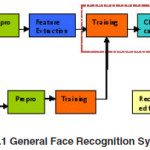
Due to the complexity of the face recognition problem, a modular approach was taken whereby the system was separated into smaller individual stages. Each stage in the designed architecture performs a intermediate task before integrating the modules into a complete system. The face recognition system developed performs three major tasks pre-processing of given face image, extracting the face feature for recognition, and performing classification for the given query sample. The system operates on two phase of operation namely training and testing phase. The functional blocks of the proposed systems is as follows → →NN Classifier

Figure 2.1 General Face Recognition Systems Click here to View figure

 

Face Recognition Using Eigen Features Overview

When designing a complex system, it is important to begin with strong foundations and reliable modules before optimizing the design to account for variations. Provided a perfectly aligned standardized database is available, the face recognition module is the most reliable stage in the system. Biggest challenge in face recognition still lies in the normalization and preprocessing of the face images so that they are suitable as input into the recognition module. Hence, the face recognition module was designed and implemented first.

Eigenface approach is one of the earliest appearance-based face recognition methods, which was developed by M. Turk and A. Pentland¹² in 1991. This method utilizes the idea of the principal component analysis and decomposes face images into a small set of characteristic feature images called eigenfaces. The eigenface method simply evaluates the entire image as a whole. These properties make this method practical in real world implementations. The basic concept behind the eigenface method is information reduction. When one evaluates even a small image, there is an incredible amount of information present. From all the possible things that could be represented in a given image, pictures of things that look like faces clearly represent a small portion of this image space. Because of this, we seek a method to break down pictures that will be better equipped to represent face images rather than images in general. To do this, we generate “base-faces” and then represent any image being analyzed by the system as a linear combination of these base faces³³.Once the base faces have been chosen we have essentially reduced the complexity of the problem from one of image analysis to a standard classification problem. Each face that wish to classify an be projected into face-space and then analyzed as a vector. A neural network approach is used for classification. The technique can be broken down into the following components:

1) Generate the eigenfaces

2) Project training data into face-space to be used with a predetermined classification method

3) Evaluate a projected test element by projecting it into face space and comparing to training data

The idea of using eigenfaces was motivated by a technique for efficiently representing pictures of faces using principal component analysis. It is argued that a collection of face images can be approximately reconstructed by storing a small collection of weights for each face and a small set of standard pictures. Therefore, if a multitude of face images can be reconstructed by weighted sum of a small collection of characteristic images, then an efficient way to learn and recognize faces might be to build the characteristic features from known face images and to recognize particular faces by comparing the feature weights needed to (approximately) reconstruct them with the weights associated with the known individuals.

The eigenfaces approach for face recognition involves the following initialization operations:[33].

1. Acquire a set of training images.

2. Calculate the eigenfaces from the training set, keeping only the best M images with the highest eigen values. These M images define the “face space”. As new faces are experienced, the eigenfaces can be updated.

3. Calculate the corresponding distribution in M-dimensional weight space for each knownindividual (training image), by projecting their face images onto the face space.

Having initialized the system, the following steps are used to recognize new face images:

1. Given an image to be recognized, calculate the eigen features of the M eigenfaces by projecting the it onto each of the eigenfaces.

2. Determined features are further processed using pca so as reduce the dimension of the image so as to have more samples since more eigenfaces will always produce greater classification accuracy, since more information is available

3. However, the eigenface paradigm, [3] which uses principal component analysis (PCA), yields projection directions that maximize the total scatter across all classes, i.e., across all face images. In choosing the projection which maximizes the total scatter, the PCA retains unwanted variations caused by lighting, facial expression,and other factors³. Accordingly, the features produced are not necessarily good for discrimination among classes. In [3], [12],the face features are acquired by using the fisherface or discriminant eigenfeature paradigm. This paradigm aims at overcoming the drawback of the eigenface paradigm by integrating Fisher’s linear discriminant (FLD) criteria, while retaining the idea of the eigenface paradigm in projecting faces from a high-dimension image space to a significantly lower-dimensional feature space.

4. These features are classified by using RBF classifier as either a known person or as unknown. The goal of using neural networks is to develop a compact internal representation of faces,which is equivalent to feature extraction. Therefore, the number of hidden neurons is less than that in either input or output layers, which results in the network encoding inputs in a smaller dimension that retains most of the important information. smaller dimension that retains most of the important information. Then, the hidden units of the neural network can serve as the input layer of another neural network to classify face images.

Principal Component Analysis

Until G. Bors and M. Gabbouj⁴ applied the Karhunen-Loeve Transform to faces, face recognition systems utilised either feature-based techniques, template matching or neural networks to perform the recognition. The groundbreaking work of Kirby and Sirovich not only resulted in a technique that efficiently represents pictures of faces using Principal Component Analysis (PCA), but also laid the foundation for the development of the “eigenface” technique of Turk and Pentland¹, which has now become a de facto standard and a common performance benchmark in face recognition .Starting with a collection of original face images, PCA aims to determine a set of orthogonal vectors that optimally represent the distribution of the data. Any face images can then be theoretically reconstructed by projections onto the new coordinate system. In search of a technique that extracts the most relevant information in a face image to form the basis vectors, Turk and Pentland proposed the eigenface approach, which effectively captures the variations within an ensemble of face images.

Calculating Eigenfaces

Mathematically, the eigenface approach uses PCA to calculate the principal components and vectors that best account for the distribution of a set of faces within the entire image space. Considering an image as being a point in a very high dimensional space, these principal components are essentially the eigenvectors of the covariance matrix of this set of face images, which Turk and Pentland¹² termed the eigenface. Each individual face can then be represented exactly by a linear combination of eigenfaces, or approximately, by a subset of “best” eigenfaces – characterized by its eigenvalues,

Let a face image be a two-dimensional N by N array of intensity values. An image may also be considered as a vector of dimension, so that a typical image of size 256 by 256 becomes a vector of dimension 65,536, or equivalently, a point in 65,536-dimensional space. An ensemble of images, then, maps to a collection of points in this huge space.face images, being similar in overall configuration, will not be randomly distributed in this huge image space and thus may be described by a relatively low dimensional subspace. The main idea of the principal component analysis is to find the vector that best account for the distribution of face images within the entire image space. These vectors define the subspace of face images, which we call “face space”. Each vector is of length N², describes an N by N image, and is a linear combination of the original face images. Because these vectors are the eigenvectors of the covariance matrix corresponding to the original face images, and they have face-like in appearance, hence referred as “eigenfaces”.

Let the training set of face images be.  The average face of the set if defined 

Figure 2.1: Mean Image Click here to View figure

 

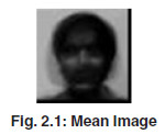
Each face differs from the average by the vector. An example training set is shown in Figure 1a, with the average face shown in Figure 1b. This set of very large vectors is then subject to principal component analysis, which seeks a set of M orthonormal vectors, , which best describes the distribution of the data. The kth vector, is chosen such that

is a maximum, subject to

The vectors and scalars are the eigenvectors and eigenvalues, respectively, of the covariance matrix

where the matrix .  The matrix C, however, is by , and determining the eigenvectors and eigenvalues is an intractable task for typical image sizes. A computationally feasible method is needed to find these eigenvectors.

If the number of data points in the image space is less than the dimension of the space (M < N²), there will be only M-1, rather than N², meaningful eigenvectors (the remaining eigenvectors will have associated eigenvalues of zero). Fortunately, we can solve for the N²-dimensional eigenvectors in this case by first solving for the eigenvectors of and M by M matrix-e.g., solving a 16 x 16 matrix rather than a 16,384 x 16,384 matrix—and then taking appropriate linear combinations of the face images Φ_n. Consider the eigenvectors υn of AT A such that

A^t AV_x = λ_x V_x   … (2.5)

Premultiplying both sides by A, we have

AA^t AV_x = λ_x AV_x     …(2.6)

from which we see that AVn are the eigenvectors of .Following this analysis, we construct the M by M matrix , where , and find the M eigenvectors of L. These vectors determine linear combinations of the M training set face images to form the eigenfaces 

Fig. 2.2: Eigen Faces

The associated eigenvalues allow us to rank the eigenvectors according to their usefulness in characterizing the variation among the images.

Feature Extraction by FLD

The PCA paradigm [3] does not provide any information for class discrimination but dimension reduction. Accordingly, the FLD[3] is applied to the projection of the set of training samples in the eigenface space. The paradigm finds an optimal subspace for classification in which the ratio of the between-class scatter and the within-class scatter is maximized.

Let the between class scatter matrix be defined as

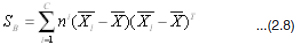
and the within-class scatter matrix be defined ass

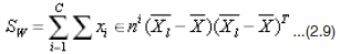
Where is the mean image of the ensemble, and is the mean image of the ith class and c is the number of classes. The optimal subspace by the FLD is determined as follows

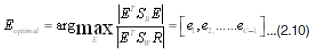
where (e1,e2,e3,…ec-1) is the set of generalized eigenvectors of SB and SW corresponding to the c-1 largest generalized eigenvalues λi=1,2,3,….c-1 i.e.

S_B E_i = λ_i S_w E_i                                       …(2.11)

Thus the feature vectors P for any query face image Z in the most discriminant sense can be calculated as follows:

P = E^T_optionalU^TZ                       …(2.12)

Face Image Classification

The eigenface images calculated from the eigenvectors of L span a basis set with which to describe face images. As mentioned before, the usefulness of eigenvectors varies according their associated eigenvalues. This suggests we pick up only the most meaningful eigenvectors and ignore the rest, in other words, the number of basis functions is further reduced from M to M’ (M’<M) and the computation is reduced as a consequence. Experiments have shown that the RMS pixel-bypixel errors in representing cropped versions of face images are about 2% with M=115 and M’=40.In practice, a smaller M’ is sufficient for identification, since accurate reconstruction of the image is not a requirement. In this framework, identification becomes a pattern recognition task. The eigenfaces span an M’ dimensional subspace of the original N² image space. The M’ most significant eigenvectors of the L matrix are chosen as those with the largest associated eigenvalues.

A new face image Γ is transformed into its eigenface components (projected onto “face space”) by a simple operation for n=1,……,M’. This describes a set of point-bypoint image multiplications and summations.

The weights form a vector that describes the contribution of each eigenface in representing the input face image, treating the eigenfaces as a basis set for face images. The vector may then be used in a standard pattern recognition algorithm to find which of a number of predefined face classes, if any, best describes the face. The simplest method for determining which face class provides the best description of an input face image is to find the face class k that minimizes the Euclidian distance where is a vector describing the face class. The face classes are calculated by averaging the results of the eigenface representation over a small number of face images (as few as one) of each individual. A face is classified as “unknown”, and optionally used to create a new face class.

Because creating the vector of weights is equivalent to projecting the original face image onto to low-dimensional face space, many images (most of them looking nothing like a face) will project onto a given pattern vector. This is not a problem for the system; however, since the distance ε between the image and the face space is simply the squared distance between the mean-adjusted input image and , its projection onto face space: .Thus there are four possibilities for an input image and its pattern vector: (1) near face space and near a face class; (2) near face space but not near a known face class; (3) distant from face space and near a face class; (4) distant from face space and not near a known face class. In the first case, an individual is recognized and identified. In the second case, an unknown individual is present. The last two cases indicate that the image is not a face image. Case three typically shows up as a false positive in most recognition systems; in this framework, however, the false recognition may be detected because of the significant distance between the image and the subspace of expected face images. So, the eigenfaces approach for face recognition could be summarized as follows:

Collect a set of characteristic face images of the known individuals. This set should include a number of images for each person, with some variation in expression and in the lighting (say four images of ten people, so M=40).

Calculate the (40 x 40) matrix L, find its eigenvectors and eigenvalues, and choose the M’ eigenvectors with the highest associated eigenvalues (let M’=10 in this example).Combine the normalized training set of images according to Eq. (6) to produce the (M’=10) eigenfaces.

For each known individual, calculate the class vector by averaging the eigenface pattern vectors [from Eq.(2.8)] calculated from the original (four) images of the individual. Choose a threshold that defines the maximum allowable distance from any face class, and a threshold θ that defines the maximum allowable distance from face space [according to Eq. (2.9)].

For each new face image to be identified, calculate its pattern vector the distance to each known class, and the distance to face space. If the minimum distance and the distance , classify the input face as the individual associated with class vector .If the minimum distance but , then the image may be classified as “unknown”, and optionally used to begin a new face class. If the new image is classified as a known individual, this image may be added to the original set of familiar face images, and the eigenfaces may be recalculated (steps 1- 4). This gives the opportunity to modify the face space as the system encounters more instances of known faces.

Results

For the implementation of face recognition a well known face database called YALE face database [31] is used. YALE face database contains 165 gray level face images of 15 persons. There are 11 images per subject, and these 11 images are, respectively, under the following different facial expression or configuration: center-light, happy, leftlight, glasses, normal, right-light, sad, sleepy, surprised, and wink. In this implementation, all images are sized to a size of 128 x 128.

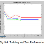
For classification or recognition purpose for the given training and test samples

Table 2.1: Result analysis for Eigen based approach Click here to View table

 

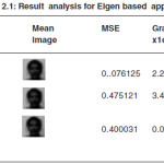
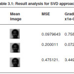
For each given input, Mean Square Error (MSE) in calculated between network output and the target vector.MSE index should have either global minimum or maximum. To find these values
Gradient decent is calculated.

Out of the 12 faces, 8 are correctly classified in the 1st match. Hence the total accuracy for the eigen feature based approach is 66.67% for illuminated affected Yale database. Thus in real time scenarios this method may be inappropriate for the illuminated affected database.

Face Recognition Using Singular Features Introduction

The singular value decomposition is a outcome of linear algebra. It plays an interesting fundamental role in many different applications. On such application is in digital image processing. SVD in digital applications provides a robust method of storing large images as smaller, more manageable square ones. This is accomplished by reproducing the original image with each succeeding nonzero singular value. Furthermore, to reduce storage size even further, images may approximated using fewer singular values.

Singular Value Decomposition

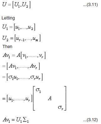
The singular value decomposition of a matrix A of m x n matrix is given in the form,

A = U∑V^T                     …(3.1)

Where U is an m x m orthogonal matrix; V an n x n orthogonal matrix, and Σ is an m x n matrix containing the singular values of A and along its main diagonal. A similar technique, known as the eigenvalue decomposition (EVD), diagonalizes matrix A, but with this case, A must be a square matrix. The EVD diagonalizes A as

A = VDV^-1                   …(3.2)

Where D is a diagonal matrix comprised of the eigenvalues, and V is a matrix whose columns contain the corresponding eigenvectors. Where Eigen value decomposition may not be possible for all facial images SVD is the result.

SVD Working Principle 

Let A be an m x n matrix. The matrix ATA is symmetric and can be diagonalized. Working with the symmetric matrix ATA, two things are true:

1. The eigenvalues of ATA will be real and nonnegative.
2. The eigenvectors will be orthogonal.

To derive two orthogonal matrices U and V that diagonalizes a m x n matrix A,First, if it is required to factor A as then the following must be true.

A^T A = (UåV^T)^T (UåV^T)
A^T A = Vå^TU^TUåV^T
A^T A = Vå^T åV^T
A^T A = Vå²V^T          … (3.3)

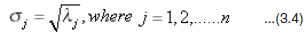
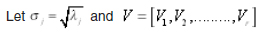
this implies that Σ2 containes the eigenvalues of ATA and V contains the corresponding eigenvectors. To find the V of the svd, rearrange the eigenvalues of ATA in order of decreasing magnitude and some eigenvalues are set equal to zero. Define the singular values of A as the square root of the corresponding eigenvalues of the matrix ATA; that is,

re-arranging the eigenvectors of ATA in the same order as their respective eigenvalues to produce the matrix

V = [V1, V2, …..Vr, Vr+1, Vr+2, …….. Vn] …(3.5)

Let the rank of A be equal to r. Then r is also the rank of ATA, which is also equal to the number of nonzero eigenvalues.

be the set of eigenvectors associated with the nonzero eigenvalues and be the set of eigenvectors associated with zero eigenvalues. It follows that:

AV₂ = (AV_r+1, AV_r+2, AV_r+n) 
AV₂ = (0, 0, …. 0)
= 0                                                                     …(3.6)

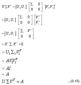
where this zero is the zero matrixes.It is defined earlier that the matrix to be the diagonal matrix with the singular values of A along its main diagonal. From above equation, each zero eigenvalue will result in a singular value equal to zero. Let be a square r x r matrix containing the nonzero singular values of A along its main diagonal. Therefore matrix Σ may be represented by:

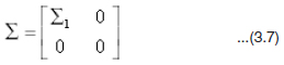
Where the singular values along the diagonal are arranged in decreasing magnitude, and the zero singular values are placed at the end of the diagonal. This new matrix Σ, with the correct dimension m x n, is padded with m – r rows of zeros and n – r columns of zeros. To find the orthogonal matrix U. Looking at the equation it follows that

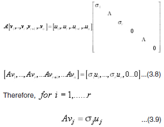
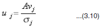
Examining above equation is a scalar value and that and is column vectors and a u j matrix vector multiplication results in another vector. Therefore, the vector resulting from the multiplication of is equal to the vector multiplied by the scalar.It could be observed at the vector as lying in the direction of the unit vector uj with absolute length . can be calculated from previously found matrix V. Therefore, the unit vector uj is a result of dividing the vector by its magnitude uj.

This Equation is restricted to the first r nonzero singular values. This allows to finding the column vectors of so long as there is no division by zero. Therefore this method allows finding only part of the matrix U. To find the other part where the singular values of A are equal to zero. As seen before in the matrix V, the matrix U may be defined as:

referring to the illustration of the four fundamental subspaces the null space of a matrix A, denotes the set of all nontrivial (non-zero) solutions to equation Ax=0. Using above equation where zero represents a zero matrix

0     …(3.13)

It follows that V2 forms a basis for the N(A) Also because

A_vj = O_uj  …(3.14)

where, The orthogonal complement to the is since the columns in the matrix V are orthogonal, the remaining vectors must lie in the subspace corresponding to the From above equation, we see that.  This equation holds the valuable information that the column vectors of U, are in the column space of A. This is because the column vectors of U are linear combinations of the columns of A. or, in matrix notation where . It now follows that and are orthogonal complements. Since the matrix U is an orthogonal matrix and the first r column vectors of U have been assigned to lie in the , then must lie in the .The vectors that lie in the are the vectors which form the matrix U2. Once matrix V is derived, the matrix Σ, and the matrix U, the singular value decomposition can be found for any matrix A. where actually does diagonalize and equal the matrix A.

The rank r is equal to the number of nonzero eigenvalues referring to four fundamental subspaces,it observed that are the eigenvectors corresponding to the nonzero eigenvalues of A, and that the remaining column vectors of V correlate with the eigenvalues equal to zero. So there exists an r nonzero singular value. Thus r is equal to the number of nonzero eigenvalues termed as rank of the matrix. These SVD features are used for facial feature decomposition to represent an image in dimensionality reduction (DR) factor. An SVD operation breaks down the matrix A into three separate matrices. because are equal to zero

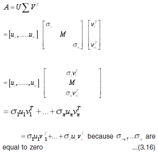
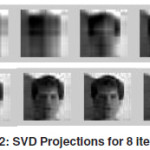
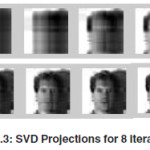
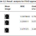
Singular values at each iteration are obtained as follows.

1. At 1st iteration SV values the facial information provided is given by
2. After n=2 iteration the facial approximationis given by,
3. After n=3 iteration the facial approximation is given by,

From the above observations it could be observed that the facial information’s are though presented in high leading images such as the eye, mouth and nose regions they are less definitive to facial expressions. So a same face image with facial variation may not be predicted in such SV approach. To overcome this limitation the SVD based face recognition approach is modified to FSVD approach as presented below.

Fractional Order Singular Value Decomposition (FSVDR)

To alleviate the facial variations on face images, a novel FSVDR is suggested. The main ideas of FSVD approach are that;

1. The weights of the leading base images should be deflated, since they are very sensitive to the great facial variations within the image matrix A itself.
2. The weights of base images corresponding to relatively small si’s should be inflated, since they may be less sensitive to the facial variations within A.
3. The order of the weights of the base images in formulating the new representation of SVD should be retained. More specifically, for each face image matrix A which has the SVD, its FSVD ‘B’ can be defined as,

B = U∑^aV^T … (3.16)

Where U, Σ and V are the SV matrices, and in order to achieve the above underlying ideas, δ is a fractional parameter that satisfies

It is seen that the rank of FSVDR ‘B’ is r, i.e., identical to the rank of A as the B matrix is fractional raised the values are inflated retaining the rank of the matrix constant.The form a set of which are similar to the base images for the SVD approach.It is observed that the intrinsic characteristic of A, the rank, is retained in the FSVD approach. In fact it has the same like base images as A, and considering the fact that these base images are the components to compose A and B, the information of A is effectively been passed to B. From the observation it could be observed that:

1. The FSVD is still like human face under lower SV.
2. The FSVD deflates the lighting condition in vision. Taking the two face images (c) and (d) under consideration, when α is set to 0.4 and 0.1, from the FSVD alone, it is difficult to tell whether the original face image matrix A is of left light on or right light on.
3. The FSVD reveals some facial details. In the original face images (a) presented, neither the right eyeball of the left face image nor the left eyeball of the right face image is visible, however, when setting α to 0.8 and 0.1 in FSVD, the eyeballs become visible.

In the case of FSVD thus the fractional parameter and it’s optimal selection is an important criterion in making the face recognition process more accurate.

Fractional Parameter ‘α’

In FSVD, α key parameter that should be adjusted. On a suitable selectivity of α parameter the recognition system can achieve superior performance to existing recognition performance. Further, in images (which are sensitive to facial variations) are deflated but meanwhile the discriminant information contained in the leading base images may be deflated. Some face images have great facial variations and are perhaps in favor of smaller ’s, while some face images have slight facial variations and might be in favor of larger α’s. The α learned from the training set is a tradeoff among all the training samples and thus is only applicable to the unknown sample from the similar distribution. Each DR method has its specific application scope, which leads to the difficulty in designing a unique α selection criterion for all the DR methods. As a result, the criterion for automatic choosing α should be dependent on the training samples, the given testing sample and the specific DR method. To optimally choose the α value minimum argument MSV criterion is used.

Mean square variance (MSV) criterion state that,

where is the standard variance of the ith class defined as

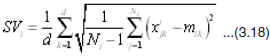
Where and respectively, denote the element of the d-dimensional samples and class mean , C is the number of classes, and i N is the number of training samples contained in the class. For an optimal selection of α value the MSV value must be optimally chosen. The smaller MSV value represents, compact the same class samples are, and on the contrary, the bigger MSV is, the looser the same class samples. When the same class samples are very loose, these samples will lead to biased estimation of the class mean, within class and between-class scatter matrices, while on the contrary, when the same class samples are compact, the estimation of the class mean, within-class and between-class variance matrices may be much more reliable. When the same class samples are compact, it is more likely that these samples can nicely depict the Gaussian distribution from which they are generated and considering the fact it is essential for the same class samples to be compact, namely MSV to be small in the recognition methods. The MSV of the training samples is given as ,

a_opt = agr min MSV (a) …(3.19)

Operational Evaluation

The FSVD based recognition approach is observed to be more effective in face recognition compared to the existing approach due to the fact that the FSVD approach works on the simple principle of deflating the more dominant leading base image (i.e. the higher order ) and inflating the lower ’s. As these lower ’s are content of low variations which are facial expressions in the given face image SV. As FSVD inflate these ’s the expression or illumination, which are completely neglected in previous, approach resulting in lower estimation accuracy are overcome in FSVD approach. The proposed FSVD based recognition approach is found to be very effective in case of intermediate feature extraction for face recognition. This feature extraction could then be used as a information for recognition systems such as PCA, LDA, NN etc. The FSVD based recognition approach is focused to overcome the effects of various real time factors in face image. Though this technique is found to inflate the low so as to reveal the expression affects this method is found to be of same computation time as compared to the existing recognition system.

When employing FSVDR as a recognition approach for face recognition method, the time complexities in training and testing are almost the same as the existing methods. The time complexity for training N samples with dimensionality is and the time complexity in testing any given unknown sample is, where C is the number of classes. For and FSVD based system it consumes in computing the FSVD for N samples where max r, c is usually smaller than N, and thus the  time complexity in training is still as with thee original recognition system, on the other hand, for any unknown sample, it takes in computing FSVD, and thus the time complexity in testing is also since is usually comparable to or less than C.

The Fractional singular value approach for face recognition involves the following initialization operations:

1. Acquire a set of training images.
2. Calculate the singular values from the training set, keeping only the best M images with the highest values. These M images define the “face space”.
3. Calculate the corresponding distribution in M-dimensional weight space for each known individual (training image), by projecting their face images onto the face space. Having initialized the system, the following steps are used to recognize new face images:
4. Given an image to be recognized, calculate the singular features of the M faces by projecting the it onto each of the faces.
5. These SVs features are raised by a fractional parameter α hence called fractional order based method. On selectivity of this parameter this recognition system can achieve superior performance by deflating the more dominant leading base features i.e. higher order SVs and inflating the lower SVs. and are tested at α = [0.5,0.8,1]6. The proposed system consist of five steps in addition to the four steps existing in the above two methods called fractional order singular value decomposition representation (FSVDR) which acts an intermediate representation between face
images and data representation for face
recognition.
7. Determined features are further processed using pca so as reduce the dimension of the image so as to have more samples since more number of samples will always produce greater classification accuracy,
8. However, principal component analysis (PCA), yields projection directions that maximize the total scatter across all classes, i.e., across all face images. In choosing the projection which maximizes the total scatter, the PCA retains unwanted variations caused by lighting, facial expression, and other factors [7].Accordingly, the features produced are not necessarily good for discrimination among classes. In [7], [8],the face features are acquired by using the fisherface or discriminant feature paradigm. This paradigm aims at overcoming the drawback of the PCA paradigm by integrating Fisher’s linear discriminant (FLD) criteria, while retaining the idea of the eigenface paradigm in projecting faces from a high-dimension image space to a significantly lowerdimensional feature space.
9. These features are classified by using RBF classifier as either a known person or as unknown.

Figure 3.1: SVD Projections for 8 iterationse Click here to View figure

 

Figure 3.2: SVD Projections for 8 iterations Click here to View figure

 

Figure 3.3: SVD Projections for 8 iterations Click here to View figure

 

Table 3.1: Result analysis for SVD approach Click here to View table

 

Figure 3.4: Training and Test Performance Click here to View figure

 

Experimental Results for Singular Value-Based Approach

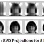
1. Singular value projection in face-space samples present in database
2. Corresponding singular value projection in face-space right side light o
3. Corresponding singular value projection in face-space left side light on
4. For this approach,12 recognition faces were randomly picked from the database, then 36 more images were used as training faces; six training faces were picked for each person with different light illumination effects.
5. Out of the 12 faces, 9 are correctly classified in the 1st match. Hence the total accuracy for the singular feature based approach is 75%Yale DB.

Figure 3.5: FSVD Projections for 8 iterations Click here to View figure

 

Figure 3.6: FSVD Projections for 8 iterations Click here to View figure

 

Figure 3.7: FSVD Projections for 8 iterations  Click here to View figure

 

Table 3.2: Result analysis for FSVD approach Click here to View table

 

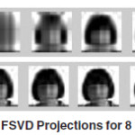
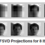
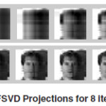
Fractional Singular Value based Approach

1. Corresponding FSV projection in face- space samples present in database at α = 1

2. Corresponding FSV projection in face-space samples having right side light on at α = 1

3. Corresponding FSV projection in face-space samples having left side light on at α = 1

From above observation it is found that at α = 1 the projected in the face spaces looks like an original images. Hence the recognition accuracy is more as compared to previous two methods 3. Out of the 12 faces, 11are correctly classified in the 1st match at α = 1.Total accuracy for the fractional singular feature based approach is 91.96% for illuminated affected Yale database.

Conclusion

The objective of this paper is to analyze developed face recognition systems. Here, the effect of environmental and surrounding effect due to illumination effect is been focused and to minimize the effect a face recognition approach is suggested.For the elimination of the additional illuminitation effects due to external surrounding effect is been also focused and is processed using singular value decomposition approach. The variation of the lighting effect could be reduced by the normalization of eigen feature values. in further improving effort the SVD approach is further improved to Fractional –SVD approach is developed.For the nono-linearlity effect of face lighting and face expression effect. The variation of these factors are observed to be effective in face recognition approach. To evaluated the performance of the developed approach a evaluation is carried out for recognition accuracy over various face images with lighting effect and expression variation. For more accurate results these systems are to analyzed thoroughly and tested different databases with different effects.

Acknowledgements

We are thankful all the authors who made available and gave an opportunity to study and analyze their papers and helped in writing this survey paper.

References

1. Jun Liu, Songcan Chen, Xiaoyang Tan “Fractional order singular value decomposition representation for face recognition” ELESVER Journal 26 March (2007).
2. Y. H. Wang, T. N. Tan and Y. Zhu “Face Verification Based on Singular Value Decomposition and Radial Basis Function Neural Network” National Laboratory of Pattern Recognition (NLPR) Institute of Automation, Chinese Academy of Sciences. networks”, IEEE Trans. Neural Networks, 13(3): 697-710.
3. Meng Joo,Shiqian Wu ,Juwei Lu and Hock Lye Toh “Face Recognition With Radial Basis Function (RBF) Neural Networks” IEEE Transactions on Neural Networks 13(3): 697(2002).
4. A. Hossein Sahoolizadeh, B. Zargham Heidari, and C. Hamid Dehghani “A New Face Recognition Method using PCA, LDA and Neural Network” International Journal of Computer Science and Engineering 2:4(2008).
5. M. Er, S. Wu, J. Lu, L.H.Toh, “face recognition with radial basis function(RBF) neural
6. P.N. Belhumeur, J.P. Hespanha, and D. J. Kriegman, “Eigen faces vs. Fisher faces: Recognition using class specific linear projection”, IEEE Trans. Pattern Anal. Machine Intel., 19: 711-720 (1997).
7. W. Zhao, R. Chellappa, A, Krishnaswamy, “Discriminant analysis of principal component for face recognition”, IEEE Trans. Pattern Anal. Machine Intel., 8 (1997).
8. M.J.Er, W.Chen, S.Wu, “High speed face recognition based on discrete cosine transform and RBF neural network”, IEEE Trans. On Neural Network, 16(3): 679,691(2005).
9. D.L. Swets and J.J. Weng”Using Discriminant Eigen features for image retrieval”, IEEE Trans. Pattern Anal. Machine Intel, 18:831-836 (1996).
10. J.J. Weng”using discriminant eigenfeatures for image retrieval”, IEEE Trans. Pattern Anal. Machine Intell., 18(8): 831-836 (1996).
11. M. Kirby, L. Sirovich, Application of the Karhunen–Loeve procedure for the characterization of human faces”,IEEE Trans. Pattern Anal. Mach. Intell. 12: 103-108(1990).
12. M. Turk, A. Pentland, “Eigenfaces for recognition”, J. Cognitive Neurosci. 3(1): 71-96 (1991).
13. J. Yang, D. Zhang, “Two-dimensional pca: a new approach to appearance-based face representation and recognition”, IEEE Trans. Pattern Anal. Mach. Intell. 26(1): 131-137(2004).
14. J.Ye, “Generalized low rank approximation of matrices”, International Conference on Machine Learning, pp. 887–894 (2004).
15. J. Liu, S. Chen, “Non-iterative generalized low rank approximation of matrices”, Pattern Recognition Lett. 27(9): 1002-1008 (2006).
16. D. Swets, J. Weng, “ Using discriminant eigenfeatures for image retrieval”,IEEE Trans. Pattern Anal. Mach. Intell. 18: 831–836(1996).
17. H. Cevikalp,M.Neamtu,M.Wilkes, A. Barkana, “ Discriminative common vectors for face recognition” , IEEE Trans. Pattern Anal. Mach. Intell. 27(1): 4-13 (2005).
18. J. Liu, S. Chen” Discriminant common vecotors versus neighbourhood components analysis and laplacianfaces: a comparative study in small sample size problem”, Image Vision Comput. 24(3): 249-262 (2006) .
19. J. Liu, S. Chen, “Resampling lda/qr and pca+lda for face recognition”, The 18th Australian Joint Conference on Artificial Intelligence, 1221–1224 (2005).
20. J. Ye, Q. Li, “ A two-stage linear discriminant analysis via qrdecomposition”, IEEE Trans. Pattern Anal. Mach. Intell. 27(6): 929–941(2005).
21. Z. Hong,”Algebraic feature extraction of image for recognition”,Pattern Recognition 24: 211-219 (1991).
22. Y. Cheng, K. Liu, J. Yang, Y. Zhuang, N. Gu, “Human face recognition method based on the statistical model of small sample size”, Intelligent Robots and Computer Vision X: Algorithms and Techniques, 85–95 (1991).
23. Y. Tian, T. Tan, Y. Wang, Y. Fang,”Do singular values contain adequate information for face recognition”, Pattern Recognition 36(3): 649-655 (2003).
24. Berk GÄokberk,”Feature-Based Pose-Invariant Face Recognition”,Bogazici University, (1999).
25. Hong,Z.,” Algebraic Feature Extraction of Image for Recognition”, Pattern Recognition, 24: 211{219 (1991).
26. Daugman, J. G., “ Complete discrete 2D Gabor transforms by neural networks for image analysis and compression”, IEEE Transactions on Acoustics, Speech, and signal Processing, Vol. 36, pp. 1169{1179, 1988.
27. Muhammad Tariq Mahmood “Face Detection by Image Discriminating”, Blekinge Institute of Technology Box 520 SE – 372 25 Ronneby Sweden
28. C.Gonzalez and Paul Wintz. “Digital Image Processing.” Addison-Wesley publishing company, second edition, (1987).
29. S.Haykin “ Neural Networks, A Comprehensive Foundation Network” Macmilla, (1994).
30. Mohammed Aleemuddin,”A Pose-Invariant Face Recognition system using Subspace Techniques”, King Fahd University of Petroleum and Minerals Dhahran, Saudi Arabia (2004).
31. Min Luo, “Eigenfaces for Face Recognition”
32. Steven Tjoa, “Statistical Pattern Recognition:Face Recognition” Dept. of Electrical and Computer Engineering, University of Maryland (2007).
33. http://cvc.yale.edu/projects/yalefaces/ yalefaces.html
34. www.dtreg.com
35. http://www.wiau.man.ac.uk/ ct.Kernel principal component analysis
36. H. Othman, T. Aboulnasr, “ A separable low complexity 2D HMM with application to face recognition” IEEE Trans. Pattern. Anal. Machie Inell., 25(10): 1229-1238 (2003).
37. K. Lee, Y. Chung, H. Byun, “SVM based face verification with feature set of small size”, Electronic letters, 38(15): 787-789 (2002).

---

This work is licensed under a Creative Commons Attribution 4.0 International License.