Introduction
In
the past decade, artificial neural networks (ANN) have been successfully used
in many areas of engineering and science.8, 24, 25 However, there
are still some problems with using this well-known method. ANN approach is a
data driven method so it is very important to select proper components of the
method based on the data in order to reach satisfactory results. Finding the
best ANN model can be considered as determination of the elements of ANN which
can be given as activation function, learning algorithm and architecture
structure.13 Determination of the best model, especially calculation
of the weights and selection of the best architecture, is still a difficult problem.3
Selection of the best architecture is a vital decision that is to determine how
many neurons should be used in the layers of a network. It is impossible to
examine all architectures and there are no general rules on how to select the
best architecture among all possible architectures.
Using
a proper architecture directly affect the performance of ANN approach.4
Therefore, determination of the best architecture is a crucial decision. In the
literature, various solution methods have been suggested to make this decision.2
Some of these methods are based on strategic algorithms such as
deletion/substitution/addition,12 polynomial time,20 constructive
and pruning21 and iterative construction19 algorithms. Another
group of selection methods are based on some kind of criteria such as weighted
information criterion,13 network information criterion18
and information entropy.23 In another group of these methods,
statistical methods such as design of experiments,9 principle
component analysis28 and Box–Jenkins analysis1, 10 are
used. Some of selection methods are based on heuristic optimization algorithms
such as genetic algorithms11 and tabu search algorithm.3 – 4
In the literature, the most widely used method is trial and error in spite of
systematic selection methods given above.2, 17 On the other hand,
trial and error is not a meticulous method and cannot guarantee to obtain a
truly optimal architecture structure.3
There
are many ANN application areas in the literature. One of these application areas
is time series forecasting.15 In this study, we also focus on time
series forecasting. However, the proposed approach can be easily used for other
application areas since it is very easy to use regression analysis. In order to
explain the proposed method better and to show the applicability of it, we
applied the proposed approach to real world time series.
Forecasting
in time series is an important issue in which many practitioners and
researchers from different fields have interested.5 In the time
series literature, various approaches range from probabilistic models to advanced
intelligent techniques have been utilized to obtain more accurate forecasts.7
In recent years, ANN approach has been one of the most preferred methods for
time series forecasting since the method has proved its success in many
forecasting applications.6 When ANN method is utilized in
forecasting, determination of the best architecture which produces the most
accurate forecasts is a vital decision. For every examined architecture, a performance
measure which is computed based on the difference between forecasts and the corresponding
observations in test set is calculated. The closer the forecasts to the
observation values, the better the architecture produces these forecasts.
According to this, the best architecture with the best performance measure value
is tried to be determined.
As
mentioned above, various efficient methods have been suggested in the
literature to solve the architecture selection problem in ANN. The most widely
used method is trial and error to determine a proper architecture since it is
not so easy to use complex algorithms of these previous methods for a specific
real world problem. This motivated us to suggest a practical and at the same
time a reliable method to determine a good architecture. This study proposes a
new architecture selection approach in which linear regression analysis is
employed to determine the best ANN architecture. The proposed approach brings a
new perspective since it combines the power of Statistics and machine learning.
When the proposed approach is used, it is possible to perform statistical
hypothesis tests. Therefore, the obtained results can be statistically evaluated
and interpreted. And, it can be statistically proved that the best architecture
is significant when the proposed approach is employed. In addition to this, it
is possible to statistically examine the effect of number of neurons on the
performance of ANN method according to the data. This is a very important
advantage provided by the proposed approach since after generating a regression
model by examining some architectures, it is possible to make inference for
other unexamined architectures without examining these ones. Statistically speaking
examined and unexamined architectures can be considered as in sample and out of
sample, respectively. Thus, computational cost of the proposed approach is very
low since it is possible to make inference for many architectures without
performing any computations. As far as I know, previous methods proposed in the
literature to solve architecture selection problem does not provide these
advantages provided by the proposed approach. To sum up, a new approach in
which statistical hypothesis tests are utilized in the selection of the best
architecture is firstly proposed in this study. In this sense, the proposed
approach brings a new perspective to ANN and provides some important advantages
such as determining the best ANN model statistically and saving time. Also, it
is easy to apply the proposed method since linear regression analysis can be easily
performed.
In
the proposed approach, while the architecture selection problem is being solved
by a statistical method of linear regression analysis, effect of number of
neurons in layers on the performance of ANN method can be statistically
evaluated by linear regression analysis. When ANN is employed to forecast time
series, the measure of the performance of ANN architectures is forecasting
error which can be computed based on the difference between forecasts and
corresponding observations in the test set. The less the forecasting error, the
better the architecture produces these forecasts. In the architecture selection
process, the aim is to determine an architecture with the minimum forecasting
error. The proposed approach is the first study in the literature that the
correlation structure between the numbers of neurons in layers and forecasting
error is statistically defined. When this correlation structure is correctly
specified by a linear regression model, it is possible to statistically show whether
or not the numbers of input or hidden neurons have a significant effect on the
forecasting performance of architectures. In regression analysis, a dependent
variable is considered to be a function of one or more independent variables.
Forecasting error and the numbers of neurons in layers are dependent and
independent variables respectively, for regression analysis in the proposed
approach. After performing linear regression analysis over some architectures,
it is possible to make inference by generated regression model. After examining
some architectures and generating a regression model, predictions can be
obtained for the performances of unexamined architectures by using this
regression model. In other words, forecasting error values of unexamined
architectures can be predicted by a significant regression model. Therefore, it
is not necessary to examine infinite number of architectures. It is already
impossible. However, it is possible to predict the performance of any
architecture when the proposed approach is utilized. This is a very important advantage
provided by the approach suggested in this study. Since computational cost of
regression analysis is very low and only a specified number of architecture is
examined, the computational cost of the proposed method is low. And, the
suggested approach is very practical and time saving.
It
is a well-known fact that the most preferred method for architecture selection
problem is trial and error because of its easy implementation. In trial and
error method, a predefined number of architecture is examined and the
architecture with the best performance is determined as the best one. On the
other hand, there is infinite number of possible architectures. An architecture
is selected among examined ones in trial and error method. When the proposed
approach is used, a predefined number of architecture is investigated and a
regression model is generated which reflects the correlation structure between
the numbers of input or hidden neurons and forecasting error of architectures.
Linear regression analysis is a well-known method and it is very easy to apply
this method. Like in trial and error method, some architectures are examined in
the proposed approach. Unlike trial and error method, it is possible to predict
the performance of any unexamined architecture when the proposed approach is utilized.
Therefore, using the proposed approach is as easy as trial and error method.
Besides, the proposed approach provides an important advantage that the
performance of any unexamined architecture can be predicted without examining
all possible architectures. Furthermore, all obtained results can be
statistically evaluated and whether or not the best architecture is significant
can be statistically shown when the proposed approach is employed.
Consequently, the proposed method is both a practical and a reliable method.
The
proposed hybrid approach is applied to three real world time series in order to
show the applicability of the method. Turkey’s Consumer Price Index (CPI),
Turkish Liras / Euro exchange rates (TL/EUR) and, the number of international
tourist arrival to Turkey (NITA) are forecasted using the proposed approach.
All obtained results are given and interpreted. As a result of the
implementation, it is shown that the proposed approach gives accurate forecasts
for these real world time series. In the next section of the paper, brief information
about ANN is given. Section 3 introduces the proposed hybrid approach. Section
4 presents the application and the obtained results. Finally, the last chapter
concludes the paper.
Artificial
Neural Networks
An artificial neural network is a mathematical model that mimics the functionalities and structure of biological neural networks.16 By training ANN models, the processes and relationships that are inherent within the data are tried to be represented.22 ANN models consist of three main elements such as learning algorithm, activation function and architecture structure. When an ANN model is constructed, it is very crucial to determine proper components of ANN according the data since ANN method is a data driven method. If these components are properly determined, the ANN model composed of these components will have a good performance.
There
are different types of architectural structures of ANN in the literature. For
example, feed forward neural networks, recurrent neural networks and multiplicative
neural networks can be given. Feed forward neural networks have been most
preferred type in the literature since it is easy to apply and they have proved
their success in many applications. Feed forward neural networks includes three
layers which are input, hidden and output layers. All of these layers include
neurons. It is possible to use more than one hidden layer in the architecture
structure. As mentioned before determining the number of neurons in these
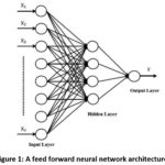
layers is called architecture selection problem. A feed forward neural network
architecture is depicted in Fig. 1. In the architecture given in Fig. 1, one
hidden layer is included. Also, this architecture has n, 4, and 1 neurons in input,
hidden and output layers, respectively. This representation can be considered
as a visual representation of a mathematical function. And, this function
represents a mathematical model. This function is generated based on the number
of neurons and activation functions used in these neurons. The data is the input
for this network. In other words, the data is the input for this function. In
Fig. 1, X1, X2, …, Xn are input values and Y
is the corresponding output value which is the output of the network. When such
an architecture is used for time series forecasting, input and output values
are lagged variables and the prediction, respectively.
Activation function performs nonlinear mapping between inputs and outputs of each neuron. Therefore, it is a key component for ANN. ANN models can learn nonlinear structures from the data by this component. In all neurons, same or different activation functions can be used. After the number of neurons and activation functions are determined, the network model is trained by using a learning algorithm. As seen from Fig. 1, all neurons in different layers are connected to each other by a weight. Direction of all connections is forward since it is a feed forward neural network. These weight values can be considered as the parameters of this mathematical model. The best output value can be obtained for the best weight values. And, the best weight values are computed by a learning algorithm. Therefore, learning algorithm is an optimization algorithm and tries to find optimum weight values in order to reach desired output values. Training algorithm has important effect on the performance of ANN method.23 Weights can be considered as parameters of the forecasting ANN model when this ANN model is applied to time series.
Other
key concepts in ANN are training and test sets. Training set represents the
part of the data which is used for training. The rest of the data can be used
as test set. The length of the training set has an effect on the training
process of the network. Observations in the test set are desired outputs or
target values. By using a performance measure, the performance of ANN model can
be evaluated over the test set. Therefore, determining the length of training
and test sets, and performance measure is also important in usage of ANN
approach. Also, the detailed information about using feed forward neural
networks in time series forecasting can be found in studies by Zhang et al.,27 and Gunay et al.,14
The
Proposed Method
As
mentioned before, ANN has some components. And, there are many options for each
of these components. It is a well-known fact that it is impossible to examine
all options for all components. Therefore, while a component is being
determined, other components can be fixed like in many studies available in the
literature.3 – 5, 9, 13 In a similar way, in the proposed approach,
some components are fixed in order to determine the best architecture. At the
same time, the proposed architecture selection method can be easily used for
any options of other components such as initial weight values, activation function,
and training algorithm. In the implementation section, the determined constants
are given when the proposed approach are applied to real time series.
In
this section, how the proposed approach can be used is clearly and simply
explained. The steps of the proposed approach can be given as follows:
Step 1: The number of architectures
which will be examined is specified.
It
is recommended that at least 50 architectures should be examined since
regression analysis can produce significant results. It can be exemplified on
an example problem in order to explain the proposed method better. Like in most
applications, let only one neuron is used in output layer. In this case, the
architecture selection problem is to determine the numbers of neurons in input
and hidden layers. For example, the number of neurons in input and hidden
layers can be changed between 1 and 12. Thus, 144 architectures are investigated.
Step 2: Initial weight values for
specified architectures are randomly generated.
It
is a well-known fact that the results obtained from the learning algorithm
depend on the initial values of weights. If the initial values are changed, the
obtained results will change. In most computer program, the initial weight values
are already determined randomly.
Step 3:
Performances of all architectures
specified in the previous step are evaluated.
A
performance measure is calculated for each architecture. For example, root mean
square error (RMSE) value can be calculated for each architecture to measure
the performance of an architecture. For 144 architectures, 144 corresponding
RMSE value is calculated.
Step 4:
Linear regression analysis is performed
and a regression model is obtained.
Performance
measure values and the numbers of neurons in the layers are dependent and
independent variables, respectively. After the regression analysis, a
regression model given below can be obtained.
yperf = β0 + β1 xinput + β2 xhidden
where yperf, xinput and xhidden represent performance measure value, the number of neurons in input layer, and the number of neurons in output layer, respectively. For example, if 144 architectures are examined, there are 144 (Xinput, Xhidden) data points (input, hidden=1,2,…,144). Each of these points represents an architecture. For instance, (2,8) represents an architecture that has 2 and 8 neurons in input and hidden layers, respectively. Also, there are 144 corresponding yperf (perf =1,2,…,144) performance measure values for all architectures. In other words, 144 RMSE values are obtained. β0, β1 and β2 coefficients are the parameters of the regression model. These coefficients are also called regression coefficients. The best values of these parameters are determined by using 144 observations.
Step 5: The significance of the
regression model generated in the previous step is tested.
The
obtained regression model should be statistically significant in order to reach
general results. By using F-test, statistical significance of the model can be
easily checked. This model explains the relation between RMSE value and the
numbers of neurons in input and hidden layers. If the regression model is not
statistically significant, return to Step 2. Otherwise, go to the next step.
Herein,
it is possible that a loop could appear if a significant regression model is
not obtained. This loop can easily be checked by adding a variable to the
algorithm. And, if a significant regression model is not obtained for a
specified number of iteration, the algorithm is terminated. This means that
there is no a significant relation between RMSE value and the numbers of
neurons in input and hidden layers. In this case, the best architecture found
so far is given as the most proper architecture. According to this, if the
regression model is not statistically significant, return to Step 2 and k = k + 1 (initial value of k is 0). If
k is less than IB, then go to the
Step 2. Otherwise, terminate the algorithm and give the best architecture found
so far as the most proper architecture. IB
is a pre-defined iteration number and its value can be specified by the user.
For example, this value can take as 50. If IB
equals to 50, this means that the algorithm goes back to Step 2 at most 50
times to obtain a significant regression model. Each time it starts from Step
2, all obtained forecasting results are changed since initial weight values for
architectures are randomly generated.
Step 6: The significance of the
coefficients of the regression model is checked.
It
is a well-known fact that at least one coefficient of the regression model is
significant if the model is significant. All coefficients are tested by using
t-test. The significant coefficients are determined. For example, if
is statistically significant, it means that
the number of neurons in input layer has a significant impact on RMSE value. In
other words, the variation in the number of neurons in input layer explains the
variation in RMSE value. As a result of this algorithm, a regression model and
the related test statistics are given. According to the information obtained
from the regression model, a proper architecture can be easily determined.
The
Implementation
In
the implementation, the proposed approach is applied to three real world time
series. These series are;
–
Monthly Turkey’s Consumer Price Index (CPI) between July 2005 and October 2013
which is taken from Turkish Statistical Institute web page,
–
Daily average values of Turkish Liras / Euro exchange rates (TL/EUR) between
30.04.2013 and 01.11.2013 which was taken from Central Bank of the Republic of
Turkey web page,
–
The monthly number of international tourist arrival to Turkey (NITA) between
June 2005 and September 2013 which was taken from Republic of Turkey Ministry
of Culture and Tourism web page.
All
time series include 100 observations. When artificial neural networks is
applied to these time series, the first 90 and the last 10 observations are
used for training and testing, respectively. The components of artificial
neural networks are explained below.
An
architecture structure of feed forward neural networks that includes one hidden
layer and one neuron in the output layer is employed. For the beginning, 144
architectures are generated by changing the number of neurons in both input and
hidden layers between 1 and 12. In other words, the number of architectures is
specified as 144.
For
neurons in hidden layer logistic activation function is used while a linear
activation function is employed for the neuron in output layer.
Levenberg-Marquardt
back propagation algorithm is used as training algorithm because of its high
convergence speed. This algorithm is already the default learning algorithm in
Matlab computer package.
RMSE criterion is used as the performance measure. The related formula of RMSE is given below.
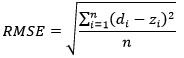
where
di and zi represent the observation
value for time i and the output value obtained from a neural network model for
time i, respectively. n is the length of the test set. Thus, n is equal to 10
in the implementation.
The
algorithm of the proposed method is coded in Matlab R2016b computer package.
And, all computations are also performed in Matlab R2016b.
Finally,
IB is taken as 5. As a result of the implementation, all obtained results are reported
in Table 1 and Table 2. In Table 1, all obtained regression models, the related
F test statistics and their probability values are given. In Table 2, 95%
confidence intervals for the coefficients b1
and b2are
presented. According to these tables, a good architecture can easily be
determined for each time series.
Table 1:
All obtained regression models
| Time Series | β0 | β1 | β2 | F test statistic | P |
| CPI | 4.958 | 0.499 | 0.269 | 7.447 | 6.61*10-4 |
| TL/EUR | 0.0254 | 0.00035 | 0.00052 | 7.899 | 4.28*10-4 |
| NITA | 1,670,691 | -24,322.6 | 26,626.84 | 4.166 | 0.016 |
According to Table 1, regression models for CPI, TL/EUR and NITA data sets are given below, respectively.
RMSECPI = 4.958 + 0.499xinput + 0.269xhidden … (1)
RMSETL/EUR = 0.0254 + 0.00035xinput + 0.00052xhidden … (2)
RMSENITA = 1670691 – 24322.6xinput + 26626.84xhidden … (3)
Table 2: Confidence Intervals
| Time Series | β1 confidence interval | | β2 confidence interval | |
| |
Lower bound
| Upper bound | Lower bound | Upper bound |
|
CPI
|
0.211
|
0.788
|
-0.019
|
0.558
|
|
TL/EUR
|
3.72*10-5
|
6.62*10-4
|
2.14*10-4
|
8.39*10-4
|
|
NITA
|
-48,878.9
|
233.7281
|
2,070.53
|
511,833.15
|
Null hypothesis for the significance of the regression model is as follows:
H0:
β0 = β1 = β2
= 0
If the related
probability value for the F test statistic is less than 0.05, the null
hypothesis is rejected. In this case, it can be said that the regression model
is significant at the 95% confidence level. When Table 1 is examined, it is
clearly seen that all obtained regression models for all time series are
significant at the 95% confidence level.
For
example, the regression model given below is obtained for CPI time series.
RMSECPI
= 4.958 + 0.499xinput + 0.269xhidden
As mentioned above, this regression model is significant at
the 95% confidence level since the probability value of F test statistic for
this model is 6.61*10-4 and it is less than 0.05. Thus, we can
statistically say that variation in RMSE can be explained by this model. Then,
the significance of the coefficients of the model should be checked. In Table
2, the 95% confidence intervals for the coefficients can be seen. These
confidence intervals for the coefficients b2
and b2
are as follows:
0.211
< β1 < 0.788
-0.019
< β2 < 0.558
b2 is not statistically significant since the 95% confidence intervals for b2 includes 0. On the other hand, it can be said that b1 is significant at the 95% confidence level. That is, variation in the number of neurons in the hidden layer is not significant in explaining variation in performance of neural networks. And, it can be statistically said that variation in RMSE can be explained by variation in the number of neurons in the input layer. According to this, any number can be used for the number of neurons in the hidden layer since it does not have an important impact on the performance of neural networks. On the other hand, if the number of neurons in input layer is increased by 1, RMSE value will increase 123.43. Therefore, using a small architecture which includes few neurons in the input layer would be wiser when CPI time series is forecasted by feed forward neural networks. In this case, it is not necessary to examine any other architectures for CPI time series since RMSE value will increase if the number of neurons in input layer is increased. In other words, an increase in the number of neurons in input layer will decrease the performance of neural network models. Therefore, there is no need to make any inference for other architectures. The best architecture among the examined 144 architectures should be used to forecast CPI time series. For CPI, this architecture is the one (3–7–1) which has 3 and 7 neurons in the input and in the hidden layers, respectively. When the proposed approach is used, it can be statistically said at the 95% confidence level that 3–7–1 architecture should be utilized to forecast CPI time series.
It
is well-known that inputs of a network are lagged variables of time series when
ANN approach is used for time series forecasting. For example, 3–7–1 means that
three lagged variables are utilized since this architecture includes three
inputs. Let Xt represents
CPI time series. Three inputs are lagged variables of CPI time series such as Xt-1,Xt-2 and Xt-3.
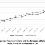
In
order to show the forecasting performance of 3–7–1 architecture for CPI, the
graph of observations and the forecasts obtained from this architecture for the
test set are depicted in Fig. 2. In this graph, vertical and horizontal axis
represent Turkey’s Consumer Price Index and dates, respectively. When this
graph is examined, it is obvious that fitness between the observations in the
test sets and the corresponding forecasts is very good. In other words, 3–7–1
architecture produces very accurate forecasts for CPI data.
Consequently,
for CPI data, it is statistically determined that 3–7–1 is the best
architecture which produces very accurate results. When CPI data is forecasted
by ANN, 3–7–1 architecture should be used. 144 architectures were examined and
the best one among them was selected as the best architecture. However, it
should be noted that by using the proposed approach, it can be statistically
said that examining 144 architectures is enough and there is no need to examine
other architectures. Also, it is visually shown that the forecasting performance
of this architecture is very good. In a similar way, the best architectures can
be easily determined for other real world time series.
As
mentioned before, when the proposed method is applied, it is possible to make
inference for architectures which is not examined. There are so many
architectures and it is not possible to examine each of them. And, there are no
general rules to determine the best architecture. This advantage of the
proposed method is very important since the performance of any unexamined
architecture can be statistically predicted without examining all possible
architectures. In order to show this feature of the proposed approach, the three
real world time series are used. RMSE values for some unexamined architecture
are calculated by using obtained regression models. Also by using same ANN
architectures, RMSE values computed over the difference between observations
and the forecasts obtained from these architectures are calculated. Then,
accuracy of RMSE values obtained from the regression models are tested by
making a comparison. As mentioned above, 144 architectures were examined by
changing the number of neurons in both input and hidden layers between 1 and
12. Therefore, an architecture which has more than 12 neurons in the hidden
layer or in the input layer was not examined. In Table 3, RMSE values obtained
from the regression model given in (1) (CPI_REG) and RMSE values obtained from
corresponding ANN architectures (CPI_ANN) are presented for some unexamined
architectures. These values were calculated for CPI time series. In Table 3,
#Input and #Hidden represent the number of neurons in input and hidden layers,
respectively.
All
architectures in Table 3 are unexamined. In other words, these architectures
are out of sample. For example, 2–17–1 architecture was not examined when
regression models were generated but it is possible to predict a RMSE value for
this architecture by using the regression model given in (1). For this
architecture, RMSE value can be easily calculated as follows:
4.959
+ 0.499 * 2 + 0269 * 17 = 10.53
When
CPI time series is forecasted by 2–17–1 architecture, RMSE value for the test
set is calculated as 10.81. However, this RMSE value can be easily predicted by
using the regression model given in (1) as above. When Table 3 is examined, it
is clearly seen that the regression model given in (1) produces very good
predictions for all out of sample architectures. These RMSE values obtained
from the regression model and ANN method are very close. For example, it can be
said that 11–13–1 architecture will produce better forecasts than those
obtained from 15–13–1 architecture without using ANN method (13.94 < 15.94).
For example, a decision maker could want to use these 14 architectures which
are out of sample. In this case, by just using the regression model in (1), it
can be said that 3–13–1 architecture should be used instead of using all of
these architectures. The reason of this is that among all these architectures,
3–13–1 architecture has the smallest RMSE prediction value (9.95). Similar
inferences can be easily made by using the regression model. It should be noted
that all this inferences are made after a statistical process. Therefore, all
of these conclusions are based on a statistical process. As mentioned before,
ANN approach was employed again in order to make a comparison to prove the
accuracy of generated regression models.
Table 3:
RMSE values obtained from the regression
model and ANN for CPI
|
#Input
|
#Hidden
|
CPI_REG
|
CPI_ANN
|
|
2
|
17
|
10.53
|
10.81
|
|
3
|
13
|
9.95
|
9.92
|
|
3
|
15
|
10.49
|
10.22
|
|
5
|
14
|
11.22
|
11.22
|
|
8
|
13
|
12.45
|
12.41
|
|
11
|
13
|
13.94
|
13.80
|
|
13
|
10
|
14.14
|
14.61
|
|
14
|
9
|
14.37
|
14.10
|
|
16
|
7
|
14.83
|
14.24
|
|
18
|
2
|
14.48
|
14.49
|
|
17
|
5
|
14.79
|
14.45
|
|
15
|
13
|
15.94
|
15.20
|
|
13
|
17
|
16.02
|
16.55
|
|
14
|
18
|
16.79
|
16.52
|
The accuracy of the regression model can also be evaluated by using statistical hypothesis tests. If the difference between the RMSE values obtained from regression model and from ANN method is not significant, it is obvious that the regression model gives accurate results for CPI data. It is possible to statistically test this difference between CPI_REG and CPI_ANN values presented in Table 3. Because of the nature of these values, Mann-Whitney U test which is a non-parametric test should be utilized. Null hypothesis for the significance of the difference is as follows:
H0: The
difference between median values of CPI_REG and of CPI_ANN is not significant
When
Mann-Whitney U test is applied, the test statistic is calculated as 92.5. And,
the corresponding probability value is 0.8 for the test statistic. Since this
probability value is greater than 0.05, the null hypothesis above is accepted.
Therefore, it can be statistically said that the difference between median values
of CPI_REG and of CPI_ANN is not significant at the 95% confidence level. In
other words, the difference between the RMSE values obtained from regression
model and from ANN method is not significant. Thus, it is possible to make
inference by just using the determined regression model for many architectures
without performing any ANN computation for CPI data. In a similar way, all test
statistics and the corresponding probability values obtained from Mann-Whitney
U test for all series are summarized in Table 4. According to Table 4, since
all probability values is greater than 0.05, the difference between the RMSE
values obtained from determined regression models given in (1), (2) and (3) and
from ANN method is not significant at the 95% confidence level. Thus, it can be
statistically said that the determined regression models produce accurate
results for all real world time series.
Table 4:
The results obtained from Mann-Whitney U
test
|
Series
|
Test Statistics
|
P
|
|
CPI
|
92.5
|
0.800
|
|
TL/EUR
|
91.5
|
0.769
|
|
NITA
|
96.0
|
0.946
|
It is also possible to examine visually the accuracy of the regression model given in (1). For these 14 out of sample architectures, the graph of the predicted RMSE values obtained from the regression model in (1) and RMSE values obtained from ANN method is given in Fig. 3 for CPI series. In this graph, vertical and horizontal axis represent RMSE values and architectures, respectively. As seen from this figure, RMSE predictions for each out of sample architecture are good. The fitness is also very good.
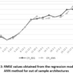 |
Figure 3: RMSE values obtained from the regression model and ANN method for out of sample architectures
Click here to View figure
|
In
a similar way, all RMSE prediction values from the regression models and
corresponding RMSE values obtained from ANN method for out of sample
architectures are presented in Table 5. In Table 5, RMSE values obtained from
ANN method are represented by TL/EUR_ANN, and NITA_ ANN for time series TL/EUR
and NITA, respectively. For each series, TL/EUR_REG and NITA_REG represent
predicted RMSE values obtained from the regression models given in (2) and (3),
respectively. In this table, #Input and #Hidden represent the number of neurons
in input and hidden layers, respectively. According to Table 5, it is obvious
that the regression models produce very good predictions for out of sample
architectures. In other words, inference ability of the proposed approach is
satisfactory.
Consequently,
it can be clearly said that applying the proposed hybrid approach to these real
world time series produces very accurate forecasts. This is an expected result
since the proposed method is based on a statistical process. In a similar way,
it is expected that the proposed hybrid approach can produce accurate results
for other real world time series because of advantages of the method.
Table 5:
RMSE values obtained from the regression
models and ANN method for some out of sample architectures
| #Input | #Hidden | TL/EUR_REG | TL/EUR_ANN | NITA_REG | NITA_ANN |
|
2
|
17
|
0.0349
| 0.0344 | 2,074,702 | 1,996,082.72 |
|
3
|
13
|
0.0332
|
0.0336
| 1,943,872 | 1,913,064.35 |
|
3
|
15
|
0.0343
| 0.0334 | 1,997,126 | 1,984,969.45 |
|
5
|
14
|
0.0344
| 0.0340 | 1,921,853 | 1,947,216.99 |
|
8
|
13
|
0.0350
|
0.0347
| 1,822,259 | 1,915,853.05 |
|
11
|
13
|
0.0360
|
0.0361
| 1,749,291 | 1,716,265.88 |
|
13
|
10
|
0.0352
|
0.0344
| 1,620,765 | 1,604,690.74 |
|
14
|
9
|
0.0350
|
0.0354
| 1,569,815 | 1,595,683.58 |
|
16
|
7
|
0.0346
| .0348 | 1,467,916 | 1,485,666.32 |
|
18
|
2
|
0.0327
| 0.0329 | 1,286,137 | 1,362,488.94 |
|
17
|
5
| 0.0340 | 0.0348 | 1,390,340 | 1,410,655.98 |
|
15
|
13
| 0.0374 | 0.0369 | 1,652,000 | 1,600,085.80 |
|
13
|
17
| 0.0388 | 0.0387 | 1,807,153 | 1,849,222.98 |
|
14
|
18
| 0.0397 | 0.0393 | 1,809,457 | 1,892,179.83 |
Conclusion
Determining
the number of neurons in the layers of a network is a vital step. A proper
architecture has to be found in order to reach good results. In the literature,
there are no general rules to find a good architecture for any data. There have
been some methods suggested to determine a good architecture but trial and
error method is still the most preferred one. This is because it is very easy
to use this method. In trial and error method, only a specified number of
architecture is examined and the architecture which has the best performance is
determined as the best one. Consequently, an architecture is selected among
examined ones although there is infinite number of possible architectures.
Therefore, this method is not reliable. In the literature, some efficient
methods have been suggested to find a good architecture. These suggested
methods are systematic and reliable. However, it is not easy to utilize most of
them because of complex algorithms of these methods. Therefore, trial and error
method is the most preferred method although it is not a systematic and a
reliable method to determine a good architecture.
In
this study, a practical and at the same time a reliable method to determine a
good architecture is proposed. The proposed architecture selection approach
which uses statistical and machine learning for determining the best ANN
architecture is suggested. It is easy to use the proposed approach since it is
very easy to utilize linear regression analysis. In addition to this, the
proposed hybrid approach combining the power of statistics and the
computational power of ANN brings a new perspective. This is because it is
possible to perform statistical hypothesis tests when the proposed approach is
employed. And, it is possible to statistically define the correlation structure
between the numbers of neurons in the layers and the performance of
architectures. Therefore, all obtained results can be statistically evaluated
and interpreted. The effects of the numbers of neurons in input or hidden
layers on forecasting performance of ANN method can be statistically evaluated
when the proposed approach is used. Also, it is possible to predict forecasting
performance of any architecture by easily using regression models instead of
using ANN architectures again and again. At the same time, this means that
computational cost of the proposed approach is very low since it is possible to
make inference for many architectures without performing complex computations.
These advantages of the proposed method are already given in the introduction
section in detail. The other solution approaches available in the literature
does not include the advantages provided by the proposed selection approach.
The
proposed approach is also applied to three real world time series in order to
show the applicability of the method. The all obtained results are presented
and discussed. As a result of the implementation, it is clearly seen that the
proposed approach produces very satisfactory and consistent forecasting results
for these real world time series.
Funding
The
author(s) received no financial support for the research, authorship, and/or
publication of this article.
Conflict of Interest
The
authors do not have any conflict of interest.
References
- Aladag C.H., Egrioglu E., Gunay S. A new architecture selection strategy in solving seasonal autoregressive time series by artificial neural networks. Hacettepe Journal of Mathematics and Statistics, 2008, 37(2): 185–200.
- Aladag C.H. Using tabu search algorithm in the selection of architecture for artificial neural networks. PhD thesis, Hacettepe University, 2009, Institute for Graduate School of Science and Engineering.
- Aladag C.H. A new architecture selection method based on tabu search for artificial neural networks. Expert Systems with Applications, 2011, 38: 3287–3293.
CrossRef - Aladag C.H. A new candidate list strategy for architecture selection in artificial neural networks. In Robert W. Nelson (ed) New developments in artificial neural networks research Nova Publisher, 2011, pp 139-150, ISBN: 978-1-61324-286-5.
- Aladag C.H. An architecture selection method based on tabu search. In Aladag CH and Egrioglu E (ed) Advances in time series forecasting, Bentham Science Publishers Ltd., 2012, pp. 88-95, eISBN: 978-1-60805-373-5.
CrossRef - Aladag C.H., Kayabasi A., Gokceoglu C. Estimation of pressuremeter modulus and limit pressure of clayey soils by various artificial neural network models. Neural Computing & Applications, 2013, 23(2): 333-339.
CrossRef - Aladag C.H., Egrioglu E., Yolcu U. Robust multilayer neural network based on median neuron model. Neural Computing & Applications, 2014, 24: 945-956.
CrossRef - Arriandiaga A., Portillo E., Sanchez J.A., Cabanes I., Pombo I. A new approach for dynamic modelling for energy consumption in the grinding process using recurrent neural networks. Neural Computing & Applications, 2015, 27(6): 1-16.
CrossRef - Balestrassi P.P., Popova E., Paiva A.P., Marangon L.J.W. Design of experiments on nn training for nonlinear time series forecasting, Neurocomputing, 2009, 72 (4-6): 1160-1178.
CrossRef - Buhamra S., Smaoui N., Gabr M. The Box–Jenkins analysis and neural networks: Prediction and time series modelling. Applied Mathematical Modeling, 2003, 27: 805–815.
CrossRef - Dam M., Saraf D.N. Design of neural networks using genetic algorithm for on-line property estimation of crude fractionator products. Computers and Chemical Engineering, 2006, 30: 722–729.
CrossRef - Durbin B., Dudoit S., Van der Laan M.J. A deletion/substitution/addition algorithm for classification neural networks, with applications to biomedical data. Journal of Statistical Planning and Inference, 2008, 138:464–488.
CrossRef - Egrioglu E., Aladag C.H., Gunay S. A new model selection strategy in artificial neural network. Applied Mathematics and Computation, 2008, 195: 591-597.
CrossRef - Gunay S., Egrioglu E., Aladag C.H. Introduction to single variable time series analysis. Hacettepe University Press, 2007, ISBN: 978-975-491-242-5.
- Gundogdu O., Egrioglu E., Aladag C.H., Yolcu U. Multiplicative neuron model artificial neural network based on Gaussian activation function. Neural Computing & Applications, 2016, Volume 27(4): 927–935.
CrossRef - Krenker J., Bešter Kos A. Introduction to the artificial neural networks. In Prof. Kenji Suzuki (ed) Artificial neural networks – methodological advances and biomedical applications, 2011, ISBN: 978-953-307-243-2, InTech, Available from: http://www.intechopen.com/books/artificial-neural-networksmethodological-advances-and-biomedical-applications/introduction-to-the-artificial-neural-networks.
CrossRef - Leahy P., Kiely G., Corcoran G. Structural optimisation and input selection of an artificial neural network for river level prediction. Journal of Hydrology, 2008, 355: 192–201.
CrossRef - Murata N., Yoshizawa S., Amari S. Network information criterion determining the number of hidden units for an artificial neural network model. IEEE Transaction on Neural Networks, 1994, 5: 865–872.
CrossRef - Rathbun T.F., Rogers S.K., DeSimo M.P., Oxley M.E. MLP iterative construction algorithm. Neurocomputing, 1997, 17: 195–216.
CrossRef - Roy A., Kim L.S., Mukhopadhyay S. A polynomial time algorithm for the construction and training of a class of multilayer perceptrons. Neural Networks, 1993, 6: 535–545.
CrossRef - Siestema J., Dow R. Neural net pruning: why and how? In Proceedings of the IEEE international conference on neural networks, 1988, (1): 325–333.
CrossRef - Solomatine D., See L.M., Abrahart R.J. Data-Driven Modelling: Concepts. In RJ Abrahart, LM See, DP Solomatine (ed) Approaches and experiences, practical hydroinformatics, Part I, 2008, Springer Berlin Heidelberg, pp 17-30. doi: 10.1007/978-3-540-79881-1_2.
CrossRef - Talaee Hosseinzadeh P. Multilayer perceptron with different training algorithms for streamflow forecasting. Neural Computing & Applications 24:695-703.
CrossRef - Yaseen Z.M., El-Shafie A., Afan HA , Hameed M, Wan Hanna Melini Wan Mohtar WHMWM, Hussain A. RBFNN versus FFNN for daily river flow forecasting at Johor River, Malaysia. Neural Computing & Applications, 2016, Volume 27(6): 1533–1542.
CrossRef - Ye J., Qiao J., Li M., Ruan X. A tabu based neural network learning algorithm. Neurocomputing, 2007, 70: 875–882.
CrossRef - Yuan H.C., Xiong F.L., Huai X.Y. A method for estimating the number of hidden neurons in feed-forward neural networks based on information entropy. Computers and Electronics in Agriculture, 2003, 40: 57–64.
CrossRef - Zhang G., Patuwo B.E., Hu Y.M. Forecasting with artificial neural networks: the state of the art. International Journal of Forecasting, 1998, 14: 35-62.
CrossRef - Zeng J., Guo H., Hu Y. Artificial neural network model for identifying taxi gross emitter from remote sensing data of vehicle emission. Journal of Environmental Sciences, 2007, 19: 427–431.
CrossRef

This work is licensed under a Creative Commons Attribution 4.0 International License.