INTRODUCTION
Computers are changing our language, our habits, our environment and in general, our lives. No longer are computer experts the only people who interact with computers each and everyday. Even, advances in information processing technology are responses to the growing need to find better, faster, cheaper, and more reliable methods of handling data, as well as searching for better ways to store and process data. Early attempts to succeed at this goal include the Abacus, Napier’s bones, Pascal and Von liebniz;s machines and Jacquard’s Punch Cards.
The new encyclopedia Britannica (2003a) described mathematics as “the science of structure, order and relation that has evolved from elementary practices of counting, measuring and describing the shapes of objects. It deals with logical reasoning and quantitative calculation, and its development has involved an increasing degree of idealization and abstraction of its subject mater.
Also, the substantive branches of mathematics are Algebra, Geometry, Numerical analysis, optimization, probability, set theory, statistics, trigonometry and more.
Sullivan (2008) defined statistics “as the science of collecting, organizing, summarizing, and analyzing information to draw conclusions or answer questions”. While Nduka (2004) defines statistics as unknown outcomes of decision making in the face of uncertainty. Further more, Emenonye and Igabari (2000) and Sullivan (2008) classified statistics into Descriptive and inferential classes. In other words, When ever statisticians use data from sample that is a subset of the population to make statement about the population, they are forming statistical inference. Thus, estimation and hypothesis testing are procedures to make statistical inferences.
Also, not to be forgotten is the fact that ‘a computerized approach” perfectly covers for the disadvantages of manual system in calculating – especially in statistical problems with enormous volume of data.
Even the new Encyclopedia Britannica (2003c) defines a computer program as a detailed plan or procedure for solving a problem with a computer; more specifically, an unambiguous, order sequence of computational instructions necessary to achieve such a solution.
“Founded in 1974, Microsoft Corporation has quickly become the largest, developer of software for microcomputers in the united state, establishing itself as a pioneer,’ states M.andell (1992) and the company has released versions of BASIC (Visual Basic) and this project report employed VB 6.0 programming language.
RESEARCH FRAMEWORK
The research work employed VB 6.0 programming language. This work produces a readable tool, for all who need knowledge of elementary hypothesis testing and also the implementation of a written program to solve problems on hypothesis testing of population mean, difference of two mean and population variance.
MEASURE OF CENTRAL TENDENCY
The mean is the most commonly used measure of location and emphasis will only be on the arithmetic Mean (x) which is defined as the sum of all individual observations of a population (or sample) divided by the total number of observations in the population (or sample). Its formulae are given below.
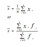
Where xr is the rth observations or rth class marks, fr is the respective frequency, n is the total number of observations, and ∑ is sigma (Greek alphabet) notation, which stands for ‘summation’.
Also, the median (me) is the value in the middle of the distribution and n is the total distribution when given ungrouped data distribution and when the total number of items, is odd, the median is the value in the (n + 1 / 2)th position. If n is even, the median is the mean of the value falling in the (n / 2)th and the (n/2 + 1)th position. That is, suppose A is the value at the (n / 2)th position, and B is the value at the (n/2 + 1)th position, the median becomes the value, A + B / 2. The median is calculated from a group data by using the formula below:
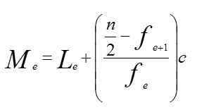
Where le is the lower boundary of the class containing the median,
fe is the frequency of the class containing the median,
fe is the cumulative frequency of the class just below the one containing the median, and ‘C’ is the class width.
CONSTRUCTION OF CONFIDENCE INTERVAL
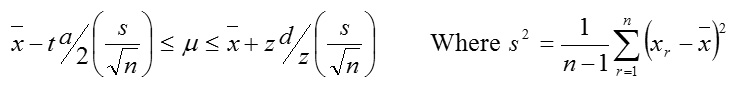
Interval estimation involves specifying a range of values on which to assert with a certain degree of confidence that some population parameter will fall within the interval. The ‘confidence’ we have that a population parameter will fall within some confidence interval (1 – α). Therefore, in order to construct a 100 (1 – α) % confidence interval for a normal population with mean μ and variance, σ2 and x ∼ N(μ,σ02) we shall consider three cases.
Case 1: Sample size is large (n≥30) and variance, σ2 is known.
we construct using 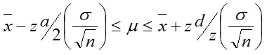
Case 2: Sample size is large (n≥30) but variance, σ2 is unknown. We construct using
Case 3: sample size is small (n≥30) and variance, σ2 is unknown.
We construct using. 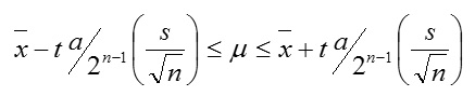
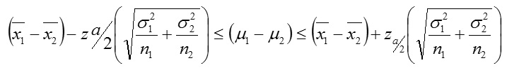
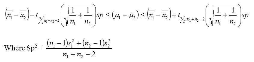
CONFIDENCE INTERVAL FOR DIFFERENCE OF TWO MEAN, μ2, μ2.
Similarly we consider three cases when the populations with samples sizes n, and n2, are normally distribution.
Case 4: Sample sizes are large (n≥30, n2, ≥30) and variances
σ12, σ22 are known.
We construct using.
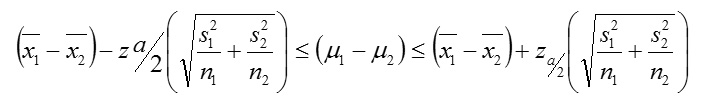
Case 5: n1, ≥30, , ≥30 and is σ12, σ22 unknown
We then construct using:
Case 6 : n≤30, n2≤, 30and variances σ12, σ22 are known
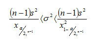
CONFIDENCE INTERVAL FOR THE VARIANCE, σ2
Given a random sample of size n from a normal population, we can construct a 100 (1-a) % confidence interval for the variance using
ELEMATARY STATICSTICAL HYPOTHSIS TESTING
Thus, a statistical hypothesis is a probability statement or conjecture about the population or populations being tested by means of sample results
HYPOTHESIS TESTING ON POPULATION MEAN
TESTING TOOLS
- Our interest may be in determining whether a population mean, μ is ‘greater then’ or ‘less than’ or ‘not equal to’ some specified value, so, we have the following.
Ho : μ = against; >, (one –tailed test)
Or ;<, (one –tailed test)
Or H: μ ≠, (two –tailed test)
(For step B of the basic procedure)
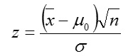
Case 7: For n ≥ 30, σ2 known, we use the statistics 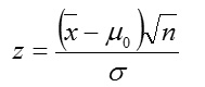
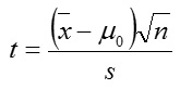
Case 8: For n ≥ 30, σ2 unknown, the statistics
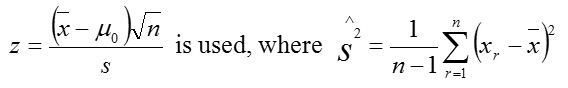
Case 9: For n ≥ 30, σ2 unknown, the statistics
 is used. (For step D the basic procedures).
Our decision is to reject for the following alternative:
Case 7: 
Case 8: The same with case 1.
Case 9: 
Where σ is the level of significance, n is the sample size, x¯ is the sample mean, μ0 is the population mean being tested for σ2 , is the population variance, and S2, is the estimate variance.
Example
- Suppose we know that that the breaking strength of a type of steel bar has a normal distribution with mean μ and variance, 25. The manufacturing process is changed as a result of research and an observed sample of breaking strength of 100 steel bars had a mean of 77.8. However, the people who conjectured that μ is above 80. Test of 1% level of significance the reliability of their proposition.
Solution
(Step A) It is a normal distribution. See first sentence of question)
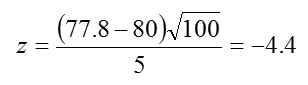
We are given that σ2 =25 (then σ = √25 = 5), n=100,
x¯ =77.8, μ0 = 80. It is obviously a case 1 problem.
(Step B) H0 : μ= 80 against H1 : μ ≠ 80 (two-tailed)
(Step C) We were given α = 1% 0.01
(Step D) since n=100 >30 and population variance is known, we use
Substituting the values in step A above,
(Step E) Since it is two-tailed, we use za/2 and α =0.01, so that a/2 = 0.05. Then z0.005 = 2.58 (Using the z table)
(Step F) /z/ > za/2 to reject H0
Since /-4.4/ = 4.4 >2.58, (As ‘/a/’means absolute)
We REJECT H0 and conclude that the means, μ does not have a mean strength of 80 as the null hypothesis states (on a 1%level of significance).
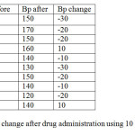
2. Consider the following data on change in blood pressure after taking a particular drug meant to lower the Bp. The hypothesis to be tested is :H0 μ ≥ 0 (that, is there is no mean Bp reduction; Bp rise ≥ 0), Ha: μ < 0 (i.e. there is a mean Bp reduction; Bp rise < 0) Ogbeibu (2005)
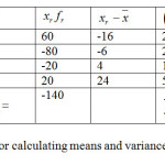
Before we start running the hypothesis testing on this question, we need a frequency distribution table from which we calculate the sample mean x¯ and variance s2 . We construct a frequency table. (See table 1.2). From this table, we have that
x¯ = -140 / 10 = -14 While s2 = 1840 / 10-1 = 204.44
(Step F) So, we have that -3.096<-2.821
That is, t 〈 ta,n-1 Implying that we Reject H0
Hence, our inference is that drug administration resulted in a significant reduction in Bp (See table 1.1 and Table 1.2).
HYPOTHESIS TESTING ON DIFFERENCE OF TWO MEAN
Here we will consider population means μx and μy. This is often referred to as the two sample problems in test of hypothesis. In this we consider two types of samples, independent samples (when faced with problems of finding out if there are any significant differences between mean and incomes of different professionals, between voting habits of men and of women, two different groups, and so on) and dependent samples (when in considering two populations, one is associated with some particular observation in the other such as data before and after treatment). Nduka (2004).
HYPOTHESIS TESTING ON POPULATION VARIANCE
As with hypothesis about population means, the test hypothesis for a single population variance can be carried out. This is a one-sample problem.
RESEARCH FRAMEWORK METHODOLOGY
Visual BASIC 6.0 was used in the design. This is because it has a lot of features like input/output instructions, arithmetic instructions, loop statement, and it runs on windows platform as well as having visual appeal.
The programming method used is modular programming which involves breaking down complex problems into independent functions and each module was tested separately before finally united by a program instruction code.
The program was tested and this involves testing the program with arbitrary values and the results generated are checked or validated to see if they are the expected output.
The project program is named “STATISTICS2007” and was specially designed to solve statistical problems like population mean, population variance, and so on.
DESCRIPTION OF “STATISTICS2007”
Visual Basic Pro CD software must be installed in your computer in order to make “STATISTICS2007” run. When it opens, click on the file with the icon labeled setup, read and follow the instructions carefully and it will be installed into your system. After which you can run STATISTICS2007 by selecting it. This will load the log in window as shown in fig 1.1.
At this stage, you are required to enter your password as well as your user ID. But if the current user is not registered, then he needs to click on the command button labeled sign up and this will load the sign up window as shown in fig 1.2: Sign up window
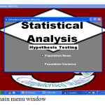
After which the user will click on the button labeled post. This will send the entry to the data Base and then take him back to the log in window to log in with his new ID. Once his ID is correct, the main menu window will now come up as shown in fig 1.3.
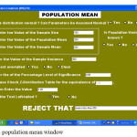
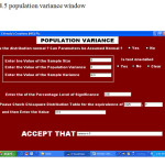
On the main menu window you have two options population mean and population variance. Double clicking on any of them will result to introducing any of the windows as shown in fig 1.4 and 1.5 respectively. This calculates the population mean window (fig1.4) and population variance window (fig1.5) respectively.
When you are through, the program takes you back to the main menu where you can exit the program or enter new data.
TEST ON THE QUALITY OF THE STATISTICA 2007
20 Novice computer users (fresh undergraduates) were used to test the friendliness of the software and, the level of usage and actualization of the right value shown that the software can be used by new university students of mathematics and computer science department.
CONCLUSION
This article will help young scientist, who needs knowledge of elementary statistical inference and how SPSS software works, in their academic training. “STATISTICS 2007”program is therefore designed to solve the population mean and population variance and can be modified to solve other statistical problems. Thus, the orderliness, simplicity, clarity, and user friendliness with which this program is written makes it user friendly, easy to use and visual appealing. Thus, it can be used in teaching students.
REFERENCES
- Emenonye, C. I. and Igabari, J. N. (2000). An outline on statistical Inference. 1st edition. Krisbec Publications, Nigeria.
- Mandell, S. L. (1992). Computer and Information Processing – concepts and Applications. 6th edition. West publishing company, USA.
- Nduka, E. C. (2004). Statistics- Concepts and Methods. 2nd edition. Crystal Publishers, Nigeria.
- The New Encyclopaedia (2003a). 15th edition Encyclopaedia Britannica Inc., USA. 7:932-933
- The New Encyclopaedia (2003b). 15th edition Encyclopaedia Britannica Inc., USA. 3:509-510.
- Sullivan III, M. (2008). Fundamentals of Statistics, Second Edition. Prentice Hall: Pearson Education, Inc. Availavle at: http://wps.pearsoncustom.com/wps/media/objects/8260/8458666/MTH340_Ch01.pdf

This work is licensed under a Creative Commons Attribution 4.0 International License.