Optical Flow Estimation Using Total Least Squares Variants

Maria A. De Jesus and Vania V. Estrela^*

Department of Telecommunications, Universidade Federal Fluminense (UFF), Rio de Janeiro, Brazil.

Corresponding author Email: vania.estrela.phd@ieee.org

DOI : http://dx.doi.org/10.13005/ojcst/10.03.03

ABSTRACT:

The problem of recursively approximating motion resulting from the Optical Flow (OF) in video thru Total Least Squares (TLS) techniques is addressed. TLS method solves an inconsistent system Gu=z , with G and z in error due to temporal/spatial derivatives, and nonlinearity, while the Ordinary Least Squares (OLS) model has noise only in z. Sources of difficulty involve the non-stationarity of the field, the ill-posedness, and the existence of noise in the data. Three ways of applying the TLS with different noise conjectures to the end problem are observed. First, the classical TLS (cTLS) is introduced, where the entries of the error matrices of each row of the augmented matrix [G;z] have zero mean and the same standard deviation. Next, the Generalized Total Least Squares (GTLS) is defined to provide a more stable solution, but it still has some problems. The Generalized Scaled TLS (GSTLS) has G and z tainted by different sources of additive zero-mean Gaussian noise and scaling [G;z] by nonsingular D and E, that is, D[G;z] E makes the errors iid with zero mean and a diagonal covariance matrix. The scaling is computed from some knowledge on the error distribution to improve the GTLS estimate. For moderate levels of additive noise, GSTLS outperforms the OLS, and the GTLS approaches. Although any TLS variant requires more computations than the OLS, it is still applicable with proper scaling of the data matrix.

KEYWORDS: Computer Vision; Inverse Problems; Motion Estimation; Optical Flow; Total Least Squares; Video Processing

Copy the following to cite this article: Jesus M. A. D, Estrela V. V. Optical Flow Estimation Using Total Least Squares Variants. Orient.J. Comp. Sci. and Technol;10(3)

Copy the following to cite this URL: Jesus M. A. D, Estrela V. V. Optical Flow Estimation Using Total Least Squares Variants. Orient. J. Comp. Sci. and Technol;10(3). Available from: http://www.computerscijournal.org/?p=6849

Intoduction

Motion Estimation in Robotics

Nowadays, robotics is receiving a lot of consideration. Robots can perform tasks in unstructured settings, assist humans, interact with users and offer their services properly. One of the key issues pertaining mobile robots is to register their position. Customarily, onboard sensors to collect environmental data for localization and mapping purposes solve this problem. Many robotic applications use procedures to appraise the robot dislocation among consecutive measurements. Matching techniques can evaluate the relative vehicle motion between two successive configurations by maximizing the similarity between the measurements acquired at each configuration.

When dealing with multimedia applications, Motion Estimation (ME) techniques can help improving compression and coding of a video sequence. For instance, the MPEG-7 offers a complete, comprehensible, and valuable collection of motion descriptors that capture the different motion characteristics in videos with a broad range of accuracy.³⁸ The fundamental goal is to give useful concise descriptors that are easy to mine and to match.

The objective of this research is to identify the Motion Vector (MV) or Displacement Vector Field (DVF) from the Optical Flow (OF) estimation via pel-recursive stationary models. These algorithms minimize the Displaced Frame Difference (DFD) in a vicinity around the working point that assumes a constant image intensity along the motion trajectory and they can provide Displacement Vectors (DVs) with sub-pixel accuracy directly with no need of transmitting the DVF.

The dislocation of each pixel between frames forms the DVF, whose estimation can be accomplished using at least two successive frames. The DVF results from the apparent motion of the pixel intensities, a.k.a. OF. The image sequence is assumed unavailable a priori, so that past data will be used as the image is processed recursively. This recursive reconstruction of the DVF requires knowledge upon the intensity values and the previously estimated DVs related to the past pixels.

Motion Estimation and Embedded Systems

OF is a widespread algorithmic computer vision tool, that is habitually used in a variety of applications like motion segmentation, Unmanned Aerial Vehicle (UAV) navigation, visual odometry, collision detection, background subtraction, tracking, and video compression to quote a few. OF can be used in areas like inspection of structures and facilities, robotics, avionics, and space activities since some of these fields have severe hardware and computational resource restrictions. Regrettably, OF computation imply in an extraordinary computational load and it involves intricate and time-consuming calculations. Furthermore, OF can be a pre-processing stage of a larger process in addition to the fact robotics, avionics and space applications usually need real-time operation.

These computational resources habitually amount to one or more general purpose CPUs (often full-embedded computers), including Digital Signal Processors (DSPs) but they are ill suited for image processing and computer vision because they lack proper special instructions and hardware sub-systems.²² Furthermore, because of their elevated clock rates, they consume a significant amount of power, which results in a bulky power supply and high heat dissipation that can be a remarkable problem.

Another difficulty with high clock rate CPUs is their vulnerability to space radiation,²³ which makes lower clock rates more appropriate. These flaws of widely existing computational hardware have made the use of OF computation techniques on lightweight, autonomous power platforms rather challenging.

There exists lots of literature on developing new methods for accurate and efficient OF computation. Several studies compared the exactitude, vector field density and computational complexity^22,23 of existing methods. Notwithstanding the developments in accuracy and the efforts to come up with numerically efficient ways, the whole computational performance of these algorithms on general-purpose CPU architectures is small, which leads to problems to implement real-time OF computation with a realistic resolution and adequate video frame rate.

While progress in OF calculation continue to appear, there has been an evident interest lately on application specific alternative computational platforms.²³ Since the software-based computation of image processing procedures is rather ineffective, in many research studies the solution is often the use of hardware acceleration.^25,26 Application Specific Integrated Circuits (ASICs) are fully custom hardware designs, usually mass-produced to fulfill the requirements of particular use regarding computational speed, space, and power consumption. The hardware can process significant amounts of data in parallelized and/or pipelined configurations in a single clock cycle while general-purpose sequential processors need a large number of clock cycles for an identical task. For that reason, ASICs are much more resourceful than traditional processors. However, ASIC design and manufacturing are long and arduous processes. Single instances of a design prototype are too costly to produce, and the answer becomes only realistic in mass fabrication. Many applications require a relatively small number of systems, which makes ASICs inappropriate. Another disadvantage of ASICs is that once a chip is factory-made, it is unmanageable to change it. Any design alteration is expensive and involves reproduction and replacement of the existing hardware. Hence, ASIC designs are only appropriate for a mass produced the mature project and are not fit for academic investigation, prototyping and/or for small amount applications.

Field Programmable Gate Arrays (FPGAs) unravel the limitations of the static structure of ASICs and can be reprogrammed several times while showing similar performance to ASICs in terms of computational speed, size, and power dissipation. This property makes FPGAs flexible platforms, which allow design alterations quickly, even the capability to be reconfigured (re-programmed) in the field. These benefits of FPGAs make them a handy platform to prototypes demanding academic studies and therefore attracted current interest for hardware-based algorithm development.

Reason to Improve Motion Estimation Algorithms

There are many alternative methods for OF computation that can be grouped as gradient-based, correlation-based, energy-based and phase-based methods.²⁴ This paper deals with gradient-based methods depend on the evaluation of spatio-temporal derivatives such as the scheme presented by Horn and Schunck²⁷ which assumed that the OF vector field is smooth and introduced a global smoothness term as a second limitation. The method from Lucas and Kanade²⁸ on the other hand, depends on a conjecture that the neighboring pixels around a current pixel move with it, indicating a locally constant flow, which brings in additional constraint equations. The answer is obtained by Ordinary Least Squares (OLS) estimation. Recently, there has been a growing interest in gradient-based methods to be implemented in embedded hardware intended for applications in robotics so that many other approaches have been proposed.^29,30,31

The prevailing OF implementations code and test algorithms on general-purpose computers.^11,12,16,39 The first inspiration is the widespread availability of such hardware and the possibility of reusing code to low requirements concerning software design experience. Another motivation is the ability to calculate the performance and compare it to existing implementations in literature. Even though PC hardware structures vary, they are standardized, and it is possible to create benchmarks. Although OF algorithms have improved over time, the PC-based implementation performance remained below the necessities of real-time applications. Alternatively, it is notorious that for many computer vision algorithms, implemented with parallelism and pipeline on FPGAs can show superior performances.²³ Regardless of the need for higher computational performance, the relative difficulty and the special expertise required resulted in few hardware implementation cases in the literature.^32,33,36

A remarkable point concerns the choice of the hardware implementation. Although this is not debated much in the existing literature, the performance of a given method on a sequential general-purpose computer does not provide a clear idea about its performance on parallelized and pipelined architectures, such as ASICs, FPGAs or Graphical Processing Units (GPUs). A particular method that does not seem efficient for a PC based implementation may have advantageous properties that make it a good candidate for a hardware-based implementation using a fixed-point representation with small word lengths.

Besides FPGAs, GPUs deliver high performance OF computation. A few studies in the collected works report the performance of OF computation on GPUs³⁴ without much discussion on its precision, and the platforms consume significant power. A GPU implementation of the Horn and Schunck’s method is presented in [35], and it uses a multi-resolution variant with two levels. In,^36,39 there is a comparison between a FPGA and a GPU implementation of OF computation using a tensor-based OF method. Nonetheless, GPUs consume considerably more power than FPGAs and need a host PC for operation. FPGAs, on the other hand, can work as a stand-alone platform. These requirements of GPUs make them impracticable for applications with severe power and space constraints such as small-scale mobile robotics.

Studies on OF computation concentrate mainly on the calculation speed. Another significant feature of a FPGA implementation that is not talked over in the existing literature is the speed-accuracy trade-off resulting from the use of fixed-point arithmetic to implement OF in FPGA hardware. Usually, using floating-point operations on FPGAs has major speed disadvantages^23,33,39 while using fixed-point decreases the accuracy of the computations. It must be pointed out that speed, power consumption, and precision are all key performance parameters to evaluate the success of an implementation.

In Section 2, the Motion Estimation Problem (MEP) is defined. The displacement vector is treated as a deterministic signal that can be estimated by means of an overdetermined system obtained from the points inside a causal neighborhood. The main principles of the computation of solutions of the DVF estimation problem by means of OLS and TLS are investigated as well as the classical Total Least Squares (cTLS) and the Generalized Total Least Squares (GTLS) are introduced in Section 3. Section 4 draws conclusions based upon the results shown in Section 3, along with the analysis of possible sources of error influencing the solution in order to introduce the Generalized Scaled Total Least Squares (GSTLS). The metrics used to evaluate the proposed algorithms are shown in Section 5. Section 6 displays some experimental results related to the application of the OLS, cTLS, GTLS, and GSTLS approaches for the clear and noise-degraded image sequences. The basic issue discussed in this Section 7 is about the applicability of the TLS variants. Finally, Section 7 summarizes the conclusions about the use of the TLS variants in Motion Estimation (ME) and Motion Compensation (MC).

Figure 1: Application of motion estimation with an Unmanned Aerial Vehicle (UAV).15  Click here to View figure

 

Figure 2: Motion as brightness change  Click here to View figure

 

The Motion Estimation Problem

Pel-Recursive Estimation

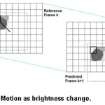
A moving pixel is one whose brightness has changed between adjacent frames. Therefore, the objective is to discover the equivalent intensity value f_k(r) of the k-th frame at position r=[x,y]^T, and d(r)=[dx,dy ]^T the corresponding ground truth for thr DV at the present point r in the current frame. The DFD is given by

△(r,d(r)) = f_k(r)-f_k-1(r–d(r))                                 (1)

and the hypothesis of perfect registration of frames produces

f_k(r) = f_k-1(r–d(r)).                                             (2)

Figure 3: Relationship between vectors u, d and do.5,9,10  Click here to View figure

 

The DFD is a function of the intensity differences and it embodies the error attribut able to the nonlinear prediction of the brightness field alongside the DV as time progresses. It is apparent from Eq. (1) that the relationship between the DVF and the evolving intensity field is nonlinear. An approximation of d(r), is found by directly minimizing △(r,d(r)) straightforwardly or by applying the Taylor series expansion off_k-1(r–d(r)) about the location (r–d^o(r)), where d^o(r) represents a forecast of d(r). This results in

Δ(r, r-d⁰(r))=Ñ^Tf_k-1(r, r-d⁰(r))u(r)+e(r, d⁰(r)),                  (3)

where u(r)=[u_x, u_y]^T=d(r)-d⁰(r) is the displacement update vector, e(r, d⁰(r)) is the truncation error associated to the higher order terms amount to the linearization error and ” = [d/dx, d/dy]^T represents the spatial gradient operator. By applying Eq. (3) to all points in a given neighborhood around the working pixel, it can be rewritten in matrix-vector form as

z = Gu + n,                                                       (4)

where the temporal gradients ∆(r, r–d^o(r)) have been piled to form vector z, matrix G is resulted from stacking the spatial gradient operators at each observation, and the remaining error terms formed the vector n. The relationship between u, d and d^o can be seen on Fig. 1.

The observation vector z contains the DFD knowledge on all the pixels in a small pre-specified causal neighborhood. Eq. (4) computes a new displacement estimate by using information contained in a neighborhood containing the current pixel. It is mentioned here that if the neighborhood has N points, then z and δz are N×1 vectors, G is an N×2 matrix and u is a 2×1 vector. Since there is always noise present in the data, matrix G and vector z in Eq. (4) are in error, that is, Eq. (4) can be rewritten as

z = (G+δG)u + δz,                                                (5)

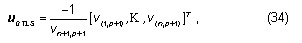
where the linearization error and the observation noise after differentiation have been combined to form δz. The spatial gradients and the interpolation are calculated as given by the next expressions.

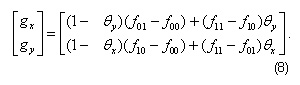
Each row of G has entries [g_x, g_y]^T corresponding to a given pixel location inside a causal mask. The spatial gradients of f_k-1 are calculated by means of a bilinear interpolation scheme (as seen on [5]). Assuming some location r=(x, y)^T and

noise after differentiation have been combined to form δz. The spatial gradients and the interpolation are calculated as given by the next expressions.

Each row of G has entries [g_x, g_y]^T corresponding to a given pixel location inside a causal mask. The spatial gradients of f_k-1 are calculated by

means of a bilinear interpolation scheme (as seen on [5]). Assuming some location r=(x, y)^T and

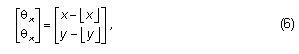
where ëxû is the largest integer that is smaller than or equal to x, the bilinear interpolated    intensity f_k-1(r) is specified by

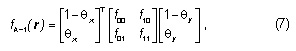
where f_ij=f_k-1(ëxû+i, ëyû+j). Eq. (7) is used for evaluating the second order spatial derivatives of f_k-1 at location r. The spatial gradient vector at r is obtained by means of backward differences in a similar way

Total Least Squares Techniques for Estimating The Dvf

Ordinary Least-Squares (OLS) Scheme

The OLS seeks to minimize the error between z and Gu like this

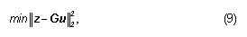
where G ∈R^m×n, z ∈R^m, m > n. The m observation is z = [z₁,…,z_m ]^T are related to the n unknown variables u = [u₁,…,u_n ]^T by

Gu = z.                                                           (10)

The OLS minimizes the sum of squared residuals ([1, 4, 9, 10, 37]) defined as

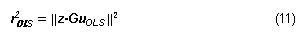
where u_OLS is the corresponding estimator. If rank(G)=r, 0<r<n, and the Singular Value Decomposition (SVD) of G becomes

then the OLS estimate in terms of the SVD of the system is

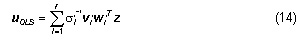
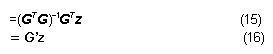
where G’ is the pseudo-inverse of G. In this case, the squared residual can be written as

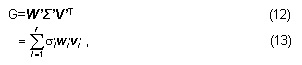
where Σ’ is a matrix that contains the singular values σ_i of G arranged in decreasing order, the columns of W’ and V’ have, respectively, their associated left singular vectors w_i and right singular vectors v_i.

Classical Total Least-Squares (cTLS) Method

The Total Least Squares (TLS) method considers the error using the distance between training points and the looked-for plane, as an alternative to the difference between the dependent variables and the estimated values for these variables), which may turn out to be proper than OLS prediction. The TLS is particularly interesting when there is a significant amount of noise in the independent variables.

The Classical Total Least-Squares (cTLS) method aims at resolving an over determined set of linear equations Ax≈b, whenever the the observation band the matrix A have errors. The system considered here comes from Eqs. (3), (4), (6), (7) and (8) (refer to^1,2,3,4,5 with errors occur in z and that G. The inherent linearity of the OLS model does not account for errors in G due to sampling, measurement, computation and modeling. The ill-posed nature of differentiation is an illustration of a possible source of errors affecting G. Hence, the cTLS error model makes it more suitable to DVF estimation than OLS.

If the perturbations δG and δz on the data [G; z] have zero mean and the covariance matrix for each of its rows is equal to the identity matrix scaled by an unknown factor (all the errors are independent and equally sized), then an exceptionally consistent estimate of the real solution of the corresponding unperturbed set is computed.

First, in order to clarify and better describe some of the possible problems related to the implementation of the cTLS technique, this work will present the cTLS method, which has unique solution associated to having a full-rank matrix [G; z]. This implies a rank reduction of [G; z] to n to

make the system Gu≈z consistent, z_cTLS will be a perturbed version of z and it will belong to the range of G. The basic cTLS looks for minimizing J(u) where

J_cTLS (u) = P[G; z] -[G_cTLS; z_cTLS] P_F²   with       (20)

z_cTLS ä Range(G_cTLS). The cTLS solution will be anyone satisfying the consistent system of equations

G_cTLSu = z_cTLS ,                                               (21)

with the associated unconstrained correction matrix given by

[∆G_cTLS; ∆z_cTLS] = [G; z] – [G_cTLS; z_cTLS].          (22)

Eqs. (20), (21), and (22) show that the augmented matrix [G; z], which contains noisy data can be approximated by a neighboring matrix [G_cTLS; z_cTLS]. This new perturbed matrix will correspond to a consistent system of equations that relies the closest to the original augmented matrix in the Frobenius norm sense. The correction matrix [∆G_cTLS; ∆z_cTLS] is the unique minimum Frobenius norm perturbation of the assumed over determined system of equations that transforms it in a consistent system of perturbed equations.

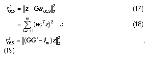
The SVD of the m´n matrix G was given in Subsection 2.2.1, and the SVD of the m´(n+1) matrix [G; z]is given by

where Σ contains the singular values s_i of [G; z] arranged in decreasing order. Matrices W and V contain, respectively, the left singular vectors , and the right singular vectors corresponding to the singular values. Then, the basic closed-form expression of the TLS solution can be given in terms of the SVD:

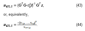
or, equivalently,

Since the last column of V corresponds to a vector belonging to the null-space of [G;z] and the cTLS solution resides in this subspace, u_cTLS is obtained from this vector after proper scaling. Eq. (26) is more useful for practical purposes than Eq. (25) because the cases where the solution is not unique are better handled by means of SVD as done by the next method.^6,7,8

Generalized Total Least Squares (GTLS)

The cTLS presents problems when all matrices are subjected to error. An extension of the generic TLS or cTLS problem, called non-generic TLS, makes the problems solvable according to.⁸ The non-generic TLS problem is still optimal concerning the TLS criteria for any number of observation vectors if additional constraints are enforced on the TLS solution space. This work will call this implementation Generalized TLS (GTLS).

The previous equations apply to the situation where matrix [G;z] is full-rank, and its singular values are different from each other. In this case, the TLS solution is unique. The necessary condition for existence and uniqueness of the GTLS solution is.^3,7,8

σ_n > σ_n+1                                                         (27)

and

v_n+1,_n+1 ≠ 0. (28)

Looking at the condition v_n+1,_n+1 ≠ 0 alone, the GTLS problem is solvable because the last column of V will belong to the null-space of [G_GTLS;z_GTLS] and Eq. (25) can be applied without problem. Generic problems have more than one solution if there is multiplicity of the smallest singular values of [G; z]. In such situations, the GTLS computes the minimum norm solution as a way of preserving uniqueness. If

σ_p>σ_p+1=…=σ_n+1,                                            (29)

with p≤n then the SVD of [G;z] is

[G; z] = WΣV^T                                                                      (30)

p = rank(G).                                                   (32)

Then, the bas ic closed-form expression of the generic TLS solution (Generalized TLS) can be given in terms of the SVD:

or, equivalently,

and the squared residual is

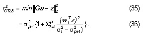
In the context of motion estimation, there are practical problems with the data caused by errors due to motion boundaries, occlusion and non-rigidity, which are known as outliers (and the TLS problem Gu ≈ z becomes non-generic or close to non-generic. Mathematically speaking, non-generic TLS problems occur whenever G is (nearly) rank-deficient or when the system Gu ≈ z is highly incompatible. is rank-deficient when its smallest singular value σ_n is approximately zero. A system Gu ≈ z is said to be highly incompatible if its smallest singular value σ_n+1 is approximately equal to σ_n . The non-generic TLS is more ill-conditioned than the full rank OLS, which implies that its solution is more sensitive to outliers. According to,^8,9,10 the difference between the squares of σ_n and σ_n+1 is a reasonable measure of how close Gu ≈ z is to the class of non-generic TLS problems. If the ratio

(σ²_n + σ²_n+1)/σ_n >1,                                                (37)

then the GTLS solution is expected to be more accurate than the OLS solution. The performance of the GTLS increases with this ratio. For non-generic TLS problems, the length of the observation vector is significant (its Frobenius norm is large), and they are close to the singular vectors w or v of G, associated with its smallest singular value. Assuming that

v_n+1,j = 0,   j=p+1,…,n+1, p < n,                        (38)

and

v_n+1,p ≠0                                                                                 (39)

the non-generic perturbed matrix is specified by

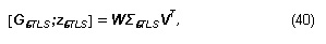
with Σ_TLS= diag(and its associated TLS correction matrix is

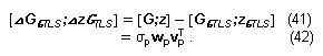
The non-generic TLS solution as defined by VanHuffel [8] is given by

Eqs. (43) and (44) correspond to a solution sought in a restricted set of right singular vectors obtained by discarding the right singular vectors associated with the smallest nonzero singular value that have a zero last component.

Relationship between the OLS and GTLS

Eqs. (16) and (43) show that the OLS and the GTLS solutions differ on a term dependent on σ_p+1, which can be used as a measure of this difference. So, the differences between them will be more pronounced as s_p+1 increases.

Eqs. (19) and (36) show that the LS technique minimizes the sum of squared residuals while the TLS approach minimizes a sum of weighted squared residuals. Starting from Eqs. (19) and (36), it can be shown that

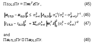
Eq. 46 shows that if PzP_F is large or if σ_n is approximately equal to s_n+1, then the GTLS will differ considerably from OLS. Eqs. (45), (46), and (47) show that if z is far from the largest singular vectors of G, then OLS will also be very different from TLS because the upper bound for this difference is proportional to Pz_OLSP_F.

Generalized Scaled Tls (Gstls) Method

A stationary DVF leads to brutal errors on regions related to borders separating objects undergoing different motions or when there is occlusion. When the GTLS is plainly applied to DVF estimation, the results are far from acceptable for reasons that will be discussed later. The number of pixels that the GTLS does not solve is greater than the amount of unsolved pixels by OLS. In order to overcome this problem, GTLS can be used in conjunction with OLS to try to process the pixels whose DVFs do not have reasonable values. Although these implementations of the GTLS did not work as well as we expected, it was noticed that when noise is involved, the participation of the OLS code decreases. The OLS alone rejects a great amount of pixels while the participation of the GTLS portion of the code increases.^13,14,17

This section aims to investigate the differences in sensitivity between the OLS and the GTLS techniques with respect to perturbations in the data to formulate a better version of the GTLS called Scaled GTLS (GSTLS). We start making some assumptions on the perturbation model used and show how it affects the TLS behavior in DVF estimation when this approach is employed without taking an error model into consideration.

The cTLS technique assumes an EIV model which considers an exact but unknown linear relationship between the variables. [G; z] are the observations of the unkown true values [G₀; z₀] and contain the measurement errors [∆G; ∆z]. The rows of [∆G; ∆z] are i.i.d. with common zero mean vector and common covariance matrix C= σ_v² I_{n+1 ,} where σ_v² is unknown. C is a positive semi definite covariance matrix.

Sensitivity Analysis of OLS and GTLS

Depending on assumptions about the noise terms, ∆G and ∆z several approaches for solving Eq. (4) can be obtained. If the entries [∆G; ∆z ] have zero mean, the same standard deviation σ_v and the covariance matrix is given by C= σ_v² I_n+1, then the GTLS gives better estimates than OLS. According to the TLS approach, G and z are perturbed appropriately so that z»Gu becomes consistent. The estimate of u in Eq. (4) corresponds to a solution of the unperturbed set [G–∆G; z–∆z ]. This first case is applicable when the linearization error is ignored, the noise statistics do not change over time, and the same differentiator is used for finding the spatial and temporal derivatives. In general, G and z are subject to different sources of error.

It should be pointed out that when the data significantly violates the EIV model assumptions, as is the case with outliers, the TLS estimates are inferior to the OLS estimates. OLS also presents stability problems (refer to Fig. 7), but they are less impressive.¹⁰ Thus, as long as the data satisfy the EIV model, the TLS will perform better than the OLS, regardless of the common error distribution and should be preferred to OLS.

Singular Values and Sensitivity of the GTLS

Since the GTLS employs the SVD of G and [G;z], the link between the singular values and the system controllability as well as stability.^7,8 The sensitivity and the invertibility of [G;z], can be quantified via the SVD and the condition number of subordinated to the L₂ norm is given by

γ =σ_MAX/σ_MIN ,                    (49)

where σ_MAX and σ_MIN are, respectively, the maximum and minimum singular values of . The above definition is a generalization of the square nonsingular case.^8,18,19 A moderate condition number guarantees that the equations are well-conditioned. Matrices with large condition numbers are said to be ill conditioned and small perturbations in the system may cause large deviations in its response (high sensitivity). An orthogonal matrix has condition number γ=1,   which is a perfect conditioning. Thus, the condition number is used as a measure of the sensitivity of the system to perturbations. Unfortunately, both the singular values and the condition number depend on the scaling of the system. σ_MIN is a measure of rank deficiency or collinearity in the system. So, it can also be regarded as a measure of invertibility. If its value is large, then the system will be less susceptible to output saturation (instability).

Some of the problems described on Section 3 were caused by errors due to the outliers resulting from motion boundaries, occlusion and non-rigidity. In the presence of outliers, the GTLS problem Gu»z becomes non-generic or close-to-non-generic. Mathematically speaking, non-generic TLS problems occur whenever G is (nearly) rank-deficient or when the system Gu»z is highly incompatible. G is rank- deficient when its smallest singular value σ_n’ is approximately zero. A system Gu»z is said to be highly incompatible if its smallest singular value σ_n+1 is approximately equal to σ_n. The nongeneric TLS is more ill conditioned than the full rank OLS, which implies that its solution is more sensitive to outliers. According to [8, 20, 21], the difference between the squares of σ_n and σ_n+1 is a reasonable measure of how close Gu=z is to the class of non-generic TLS problems. If the ratio (σ_n – σ_n+1 )/σ_n > 1 holds, then the GTLS solution is expected to be more accurate than the OLS solution. The performance of the TLS increases with this ratio. For non-generic TLS problems, the length of observation vector z is large (the Frobenius norm of z is large) and they are close to the singular vectors w or v of G, associated with its smallest singular value.

Scaling

C does not have the form σ_v²I, because the z and G are corrupted by different errors. G involves the calculation of spatial derivatives while z corresponds to the temporal gradients that are initially set equal to the frame difference. However, both are affected by noise. In the subsequent analysis, G and z are modeled as being contaminated by additive zero-mean Gaussian noise with variances equal to σ_G² and σ_z², respectively, which disturbs Gu=z.

The distributions of g_x and g_y can be calculated by means of Eq. (8) and the following facts:

The image pixels are corrupted by i.i.d. noise, with Gaussian distribution, zero mean and variance σ_S².

0≤ (1– θ_y)≤ 1 and 0≤ (1– θ_x)≤ 1 as in Eq. (6).

The moment generating function of a random variable Z=X–Y, where X and Y are zero-mean normally distributed random variables with variances σ_x² and σ_y², respectively, is ϕ(t) =exp[(σ_x² +σ_y²)/2]. It turns out that both are zero-mean normally distributed with variances σ_gx² = 2σ_S²(1-2θ_y+ θ_y²), and

σ_gy² = 2σ_S²(1-2 θ_x+ θ_x²).

Now, the covariance matrix of each row of the augmented matrix [G; z] can be written as

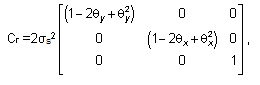
where the values of θ_x and θ_y were considered constant. An important consequence of Gu = z is the fact that C_r is different from the TLS assumption of a covariance matrix equal to C =σ²I_n+1,n+1. This explains part of the problems described in Section 3. Each row of [G; z] has its corresponding error matrix C_r ≈ C_iⁱ, i=1,…,m. In general, those matrices are different because of the different θ_x’s and θ_y’s involved. One way of overcoming this problem is to pre-and post-multiply [ΔG;Δz] by matrices D and E, respectively, leading to the desired distribution of errors with C=σ_k²I_n+1,n+1. as follows:

C_r = [ΔG;Δz] [ΔG;Δz]^T = [ΔG’;Δz’] [ΔG’;Δz’]^T

= D[ΔG;Δz]E = σ_k²I_n+1,n+1,

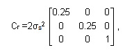
where is some constant. It can be shown that the same transformation is induced in the augmented matrix [G;z] and the TLS technique can be applied to the new scaled system [G’;z’] = D[G; z]E, so that its entries are corrected according to the errors in [ΔG;Δz], then a transformation, such that D[ΔG;Δz]E = [ΔG’;Δz’]. This problem is very difficult to solve due to the need of equilibrating all the rows of [G; z] at the same time. To avoid this, smoothness will be assumed which leads to similar deviations for the pixels in the mask. So, θ_x ≈θ_y ≈0.5 can be used with C_r ≈ C_iⁱ, i=1,…,m and

[G’;z’] = D[G; z]E.

The GTLS does not assume any knowledge on the error distribution of [ΔG;Δz] and it implies that all entries of G and z are affected by uncorrelated, equally sized errors. The GTLS estimate will be inconsistent, if this assumption is violated. Considering the distribution of errors of [ΔG;Δz] and transforming [G;z] conveniently leads to an improved error covariance C and it handles the unlikely situation of no error.

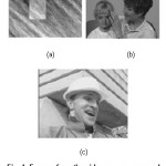Figure 4: Frames from the video sequences used for tests: (a) Synthetic frames, (b) Mother and Daughter and (c) Foreman. Click here to View figure

 

Metrics To Evaluate The Experiments

The quality of the motion field is assessed using the metrics^2,3 discussed below when applied to the video sequences displayed in Fig. 4.

Mean Squared Error (MSE)

The MSE indicates the degree of similarity of the OF among the estimates and the ground truth of adjacent frames from sequences with well-known motion. We can calculate the MSE in the horizontal direction MSE_x and in the vertical direction MSE_y like this

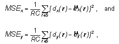
pixel coordinates, R and C are, in that order, the number of rows and columns in a frame, d(r)=(d_x(r), d_y(r)) is the genuine DV at r, and d̂(r)=(d̂_x(r), d̂_y(r)) its estimation.

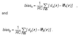
Bias

The bias establishes the correspondence degree between the estimated and the original OF and it amounts to the average of the difference between the true and estimated DVs for all pixels within a frame S, and it is defined alongside the x and y directions as

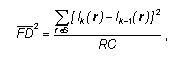
Mean-squared Displaced Frame Difference

This metric ponders the comportment of the average of  the Squared Displaced Frame Difference —2/DFD It represents an evaluation of the progress of the intensity gradient with time as the sequence develops by probing the squared difference between the present brightness I_k(r) and its predicted value I_k-1(r-d(r)).In ideal circumstances, the 2/DFD is zero, meaning that all motion was identified correctly (I_k(r)= I_k-1(r-d(r) for all r’s). In practice, the must be small, and it is defined as 

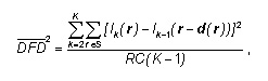
with K representing the video length in frames.

Improvement in Motion Compensation

The average Improvement in Motion Compensation —IMC(dB) between two consecutive frames is given by

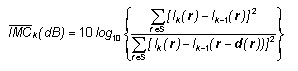
where S is the frame under analysis. It expresses the ratio in decibel (dB) between the mean-squared frame difference —2/FD defined by

and the —2/DFD between frames k and (k–1). As far as the use of this metric goes, we chose to apply it to a sequence of K frames, resulting in the following equation for the average improvement in motion compensation:

Figure 5: Errors for the noiseless Synthetic sequence: (a) OLS, (b) GTLS, and (c) GSTLS  Click here to View figure

 

Figure 6: Errors for the Synthetic sequence with SNR = 20dB: (a) OLS, (b) GTLS, and (c) GSTLS.   Click here to View figure

 

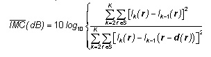
When it comes to ME/MC (dB). If motion can be detected without any error, then the denominator of the preceding expression would be zero (perfect registration of motion) thus leading to —IMC (dB)=.

Experiments and Discussion

Several experimental results that exemplify the effectiveness of the GTLS and the GSTLS approaches when compared to the OLS. All video sequences are 144×176 pixels, 8-bit (QCIF format). The algorithms were applied to three image sequences: one synthetically produced, with known movement; the “Mother and Daughter” (MD) and the “Foreman” (FM). For each video sequence, two types of experiments were done: one for the noiseless case and the other for a sequence whose frames are corrupted by a Signal-to-Noise-Ratio SNR = 10log₁₀ [σ²/ σ_c²], with σ² is the variance of the original image and σ_c² is the variance of the noise-corrupted image.^9,10

Table 1: Results for different implementations, SNR = ∞ (noiseless).   Click here to View table

 

Table 2: Results for different implementations, SNR =20dB  Click here to View table

 

Experiment 1

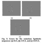
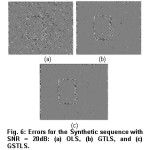
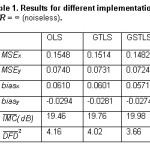
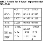
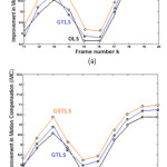
This sequence has a diagonally moving rectangle immersed in a changing background. All the background pixels move to the right. Table 1 lists the values for the MSEs, biases, —2/DFD and —IMC (dB) for the estimated OF obtained with the OLS, GTLS, and GSTLS methods in the absence of noise. All the algorithms employing the TLS show improvement in terms of the metrics used. When we compare TLS algorithms with the OLS, we see that the improvements are small. Table 1 and Table 2 show the values for the MSEs, —2/DFD and —IMC for the estimated OF using the OLS, GTLS, and GSTLS techniques for noiseless and noisy frames (SNR = 20dB ) of the Synthetic sequence, respectively. The results for both cases present better values of  —IMC (dB) and —2/DFDas well as MSEs and biases for all procedures using the TLS. The best results regarding metrics and visually speaking are obtained with the GSTLS algorithm. For the noisy case, it should be pointed out the substantial drop of the noise interference when it comes to the background and the object motion. For this algorithm, even the movement around the borders of the rectangle is clearer than when the OLS estimator is used.

Figure 7 Click here to View figure

 

Figure 8 Click here to View figure

 

Experiment 2

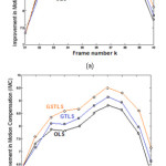
Fig. 7 presents the qualitative performance in terms of the plots for frames 31-40 of the noiseless and noisy (SNR = 20dB ) cases of the MD video sequence, for all algorithms implemented. The best performance comes from the GSTLS algorithm, which provides, on the average, higher values than the OLS and GTLS procedures for the noiseless case. For the noisy case, the values are not as high as in the earlier situation. By visual inspection, the noise-free case does present dramatic differences between motion fields. For the noisy case, we were able of capturing the rotation of the mother’s head, although inappropriate displacement vectors were found in regions where there is no texture at all such as the background, for instance, there is less noise than when the OLS is used.

Experiment 3

Fig. 8 demonstrates results achieved for frames 11-20 of the “Foreman” sequence, which has frames with abrupt motion. The algorithms relying on TLS outperform the OLS method. This sequence has shown very good values for both the noiseless and the noisy cases. By looking at the error plots in the motion compensated frames, the procedure GSTLS performs better than the OLS and the GTLS visually speaking.

Conclusion

This investigation attacks some concerns related to the usance of adaptive pel-recursive procedures to solve the problem of estimating the DVF. We analyzed the problem of robust estimation of the DVF between two consecutive frames, concentrating our attention on the noise effect on the estimates. The observation z is subjected to independent identically distributed (i.i.d.) zero-mean additive Gaussian noise n. This entire paper looked at n and the update vector u as the only random signals de facto, as well as z since it arises from a linear combination of u and n. Robustness to noise can be accomplished with regularization and by making the regularization parameters dependent on data.^5,9,10,37

The motion features offer the easiest knowledge on the temporal dimension of a video sequence and influence significantly tasks such as video indexing. Camera motion-estimation procedures, trajectory-matching methods, and aggregated motion vector histogram-based techniques form the core of past work in video indexing using motion characteristics.³⁹

The motivation behind this research is the lack of a suitable hardware that is capable of computing OF vector field in real time for the deployment of computer vision in robots since low-power real-time performance is of particular importance for mobile robotic platforms. Another important aspect for a full OF implementation is pre-processing.

This work aims at the minimization of the DFD at each pixel with respect to u, based on an initial DVF estimate. Therefore, an estimate of the DV d results from knowledge of the initial estimate and an update vector. The simplest manner to solve this problem is by means of an OLS solution that assumes errors only on one column of the augmented matrix associated to the overdetermined system resulting from the DVF estimation problem. Earlier works such as¹ considered u was a sample of a stochastic process and added a term that accounted for truncation error (Wiener-based or OLS pel-recursive algorithm). The covariance matrices were chosen equal to σ_u² and σ_v²I, respectively, where represents the identity matrix. In Section 3, it was shown that the application of the GTLS does present some improvement when compared to the approaches mentioned in the previous paragraph due to instability problems of the TLS technique. In Section 4, the GSTLS estimator that better uses the characteristics and advantages of the TLS technique was developed. It models the covariance matrix associated with the errors in each row of the augmented matrix. In order to do so, the error noise on each pixel is assumed normally distributed with mean zero. Then, the errors in the entries of G are estimated based on pixel noise and considering functions of random variables. Since the resulting perturbed data covariance matrices no longer have the form σ_v²I, the data can be transformed, so that each row has an error covariance matrix diagonal with equal error variances. This means that the basic assumption of the classical TLS is now valid. This procedure is referred as scaling. When a solution of the transformed set of equations is found, it must be converted back to a solution of the original set of equations.^{8,13,14,17,18}

A spatially-adaptive approach was used, and it consists of using a set of masks, each one representing a different neighborhood and yielding a distinct estimate. The final estimate is the one that provided the smallest DFD. The results from some experiments demonstrated the advantages of employing multiple masks.^5,9,10

Still, the technique has some drawbacks.^4,8,13,14 Serious trouble emerges when measuring variables with different units. First, consider determining the distance between a data point and a curve. More specifically, what are the units for this distance? If a distance is measured based on the Pythagoras’ theorem, then it is clear that the estimation involves quantities measured in different units, and as a result, this leads to worthless outcomes. Secondly, after rescaling one of the variables, then different outcomes (and a different curve) may result. Dimensionless variables can remediate the incommensurability problem. This is called normalization or standardization. Nevertheless, these procedures may lead to fit models that are not equivalent to each other. One line of attack is normalization by a known (or an estimated) factor followed by the minimization of the Mahalanobis’ distance between the points and the line, which provides a maximum-likelihood solution. The analysis of variances can provide the unknown precision.

In short, cTLS and GTLS vary according to the units used, i.e., they are scale variant. For a more exact model, this property must be enforced. Using multiplication instead of addition allows combining residuals (distances) obtained in different units. Cogitate the problem of fitting a line through data points. The multiplication result of the vertical and horizontal residuals is twofold the area of the triangle whose frontiers are the residual lines and the fit line. A better option is the line, which minimizes the sum of these areas.

A thought-provoking problem currently under investigation is to devise a more intelligent way of selecting the neighborhoods upon which to build systems of equations and how to handle the information on smooth events in a scene. Better regularization strategies can improve the estimates obtained with TLS variants.

References

1. Biemond, J., Looijenga, L., Boekee, D. E. and Plompen, R.H.J.M. A pel-recursive Wiener-based displacement estimation algorithm. Sig. Proc.1987;13:399-412.
2. Mesarovic, V.Z., Galatsanos N.P. and Katsaggelos A.K. Regularized constrained total least squares image restoration. IEEE Trans Im. Proc.1995;4(8):1096-1108. doi: 10.1109/83.403444
3. Cadzow,  J. C. Total least squares, matrix enhancement, and signal processing. Digital Sig. Proc.1984;4:21-39.
4. Tsai, C.J., Galatsanos, N.P., Stathaki, T. and Katsaggelos, A. K. Total least-squares disparity-assisted stereo optical flow estimation. Proc. IEEE Im. Multidimensional Dig. Signal Proc. Work.1999.
5. Estrela, V. V., Rivera, L. A., Beggio, P.C. and Lopes, R. T. Regularized pel-recursive motion estimation using generalized cross-validation and spatial adaptation. Proc. of the SIBGRAPI 2003 – XVI Brazilian Symp. on Comp. Graphics and Im. Proc.2003;doi: 10.1109/SIBGRA.2003.1241027
6. Golub G.H. and Van Loan. C.F. An analysis of the total least squares problem. SIAM J. Numer. Anal.1980; 17:883-893.
7. Golub, G.H. and Van Loan, C.F. Matrix Computations. Johns Hopkins University, Maryland.1989.
8. Van Huffel, S. and Vanderwalle. J. The Total Least Squares Problem: Computational Aspects and Analysis. SIAM, 1991; Philadelphia.
9. Coelho, A.M. and Estrela, V. V. Data-driven motion estimation with spatial adaptation. Int’l J. of Image Proc. (IJIP).2012;6(1):54. doi: citeulike-article-id:11966066
10. Coelho, A. M. and Estrela, V. V. A study on the effect of regularization matrices in motion estimation. Int’l J. of Comp. Applications.2012;51(19):17-24. doi: 10.5120/8151-1886
11. Coelho, A. M. and Estrela, Vania V. EM-based mixture models applied to video event detection. In Principal Component Analysis – Engineering Applications (Parinya Sanguansat, P. ed). Intech Open, 2012; pp. 101-124. ISBN 978-953-51-0182-6, 2012 doi: 10.5772/38129
12. Marins, H. R. and Estrela, V. V., On the Use of Motion Vectors for 2D and 3D Error Concealment in H.264/AVC Video. In Feature Detectors and Motion Detection in Video Processing (Dey, N., Ashour, A., Patra, P. K. eds). IGI Global, 2017; pp. 164-186. doi: 10.4018/978-1-5225-1025-3.ch008
13. Fang, X. Weighted total least squares: necessary and sufficient conditions, fixed and random parameters. J. Geod.2013;87(8):733–749.
14. Grafarend, E. and Awange, J. L. Applications of Linear and Nonlinear Models, Fixed Effects, Random Effects, and Total Least Squares.2012. Springer, Berlin.
15. Leick, A. GPS Satellite Surveying. Wiley, New York. 2004.
16. Li, B., Shen, Y. and Lou, L. Seamless multivariate affine error-in-variables transformation and its application to map rectification. Int. J. GIS.2013;27(8):1572–1592.
17. Neitzel, F. Generalization of total least-squares on example of unweighted and weighted 2D similarity transformation. J. Geod. 2010.84:751–762.
18. Schaffrin, B. and Felus, Y. On the multivariate total least-squares approach to empirical coordinate transformations: Three algorithms. J. Geod. 2008;82:373–383.
19. Schaffrin, B. and Wieser, A. On weighted total least-squares adjustment for linear regression. J. Geod.  2008; 82:415–421.
20. Shen, Y., Li, B.F. and Chen, Y. An iterative solution of weighted total least-squares adjustment. J. Geod. 2010; 85:229–238.
21. Xu, P.L., Liu, J.N. and Shi, C. Total least squares adjustment in partial errors-in-variables models: algorithm and statistical analysis. J. Geod. 2012;86(8):661–675.
22. Gultekin, G. K. and Saranli, A. An FPGA based high performance optical flow hardware design for computer vision applications. Microproc. & Microsystems. 2013;37(3):270-286. doi: 10.1016/j.micpro.2013.01.001
23. Komorkiewicz, M., Kryjak, T. and Gorgon, M. Efficient hardware implementation of the Horn-Schunck algorithm for high-resolution real-time dense optical flow sensor. Sensors. 14(2):2860–2891. http://doi.org/10.3390/s140202860
24. Barron, J., Fleet, D. and Beauchemin, S. Performance of optical flow techniques. Int’l J. of Comp. Vision (IJCV).1994; 12:43-77.
25. Chien, S.-Y. and Chen, L.-G. Reconfigurable morphological image processing accelerator for video object segmentation, J. of Sig. Proc. Systems. 2011;62:77-96.
26. Lopich, A. and Dudek, P. Hardware implementation of skeletonization algorithm for parallel asynchronous image processing. J. of Sig. Proc. Systems. 2009;56:91-103.
27. Horn, B. and Schunck, B. Determining optical flow. A.I.1981;17:185-203.
28. Lucas, B. and T. Kanade, T. An iterative image registration technique with an application to stereo vision. Proc. of Imaging Understand. Workshop.1981;121–130.
29. Nagel, H.-H. On a constraint equation for the estimation of displacement rates in image sequences. IEEE Trans. on Patt. Anal. and Mach. Intellig.1989;11:13-30.
30. Black, M. and Anandan, P. A framework for the robust estimation of optical flow. Proc. of the 4^th Int’l Conf. on Comp. Vision.1993;231–236.
31. Proesmans, M., van Gool, L., Pauwels, E. and Oosterlinck, A. Determination of optical flow and its discontinuities using non-linear diffusion. Proc. of the 1994 Europ. Conf. on Comp. Vision.1994;295–304.
32. Niitsuma, H. and Maruyama, T. High-speed computation of the optical flow. Proc. of the Int’l Conf. on Image Analysis and Proc. (ICIAP).2005;287–295.
33. Shibuya, L. H., Sato, S. S., Saotome, O. and Nicodemos, F. G. A real-time system based on FPGA to measure the transition time between tasks in a RTOS. Proc. of the 1^st Work. on Embedded Syst.2010; 29-39. ​​http://sbrc2010.inf.ufrgs.br/anais/data/pdf/wse/st01_03_wse.pdf
34. Strzodka, R. and Garbe, C. Real-time motion estimation and visualization on graphics cards. Proc. of the 2004 Conf. on Visualization.2004;545–552.
35. Mizukami, Y. and Tadamura, K. Optical flow computation on compute unified device architecture. Proc. of the 14th Int’l Conf. on Image Analysis and Proc.2007;179–184.
36. Chase, J., Nelson, B., Bodily, J., Wei, Z. and Lee, D.-J. Real-time optical flow calculations on FPGA and GPU architectures: a comparison study. Proc. of the 16^th Int’l Symp. on Field-Programmable Custom Comp. Machines.2008;173–182.
37. Yu, J. J., Harley, A. W. and Derpanis. K. G. Back to basics: Unsupervised learning of optical flow via brightness constancy and motion smoothness. arXiv preprint arXiv:1608.05842, 2016.
38. MPEG-7 Overview, ISO/IEC JTC1/SC29/WG11 WG11N6828, 2004.
39. Popovic, V., Seyid, K., Cogal, Ö., Akin, A., and Leblebici, Y. Real-time image registration via optical flow calculation. Design and Implementation of Real-Time Multi-Sensor Vision Systems.2017; Springer, Cham.   doi: 10.1007/978-3-319-59057-

---

This work is licensed under a Creative Commons Attribution 4.0 International License.