Assessment of Accuracy Enhancement of Back Propagation Algorithm by Training the Model using Deep Learning

Baby Kahkeshan and Syed Imtiyaz Hassan

Department of Computer Science & Engineering, Jamia Hamdard, New Delhi, India.

 

Corresponding author Email: s.imtiyaz@gmail.com

DOI : http://dx.doi.org/10.13005/ojcst/10.02.07

ABSTRACT:

Deep learning is a branch of machine learning which is recently gaining a lot of attention due to its efficiency in solving a number of AI problems. The aim of this research is to assess the accuracy enhancement by using deep learning in back propagation algorithm. For this purpose, two techniques has been used. In the first technique, simple back propagation algorithm is used and the designed model is tested for accuracy. In the second technique, the model is first trained using deep learning via deep belief nets to make it learn and improve its parameters values and then back propagation is used over it. The advantage of softmax function is used in both the methods. Both the methods have been tested over images of handwritten digits and accuracy is then calculated. It has been observed that there is a significant increase in the accuracy of the model if we apply deep learning for training purpose.

KEYWORDS: Machine Learning; Deep Learning; Deep Belief Nets; Back Propagation; Restricted Boltzmann Machines; Artificial Neural Networks; Softmax function

Copy the following to cite this article: Kahkeshan B, Hassan S. I. Assessment of Accuracy Enhancement of Back Propagation Algorithm by Training the Model using Deep Learning. Orient.J. Comp. Sci. and Technol;10(2)

Copy the following to cite this URL: Kahkeshan B, Hassan S. I. Assessment of Accuracy Enhancement of Back Propagation Algorithm by Training the Model using Deep Learning. Orient. J. Comp. Sci. and Technol;10(2). Available from: http://www.computerscijournal.org/?p=5544

Introduction

Deep learning is a branch of the rapidly growing field of machine learning. Machine learning is a field of computer science which makes use of AI concepts, to enable computers to learn from problem solutions and make use of the knowledge for new problems. Machine learning have proven useful in a mining structured, semi-structured and unstructured data. The values generated by this process may be applied in various fields as reported in [1, 2, 3, 4]. Handwritten digit recognition is the capability of an automated system to recognize digits written by various human hands and has its applications in bank checks details recognition, zip codes recognition and others. This research proposes a solution for the same using deep learning and back propagation algorithms. An artificial neural network has been built for this purpose and then tested with the required algorithms. For the purpose of validation, MNIST data set [5] of handwritten digits has been used.

This paper explores the applicability of deep learning in handwritten digit recognition system. The proposed solution in this research makes use of deep belief nets.

Background

A brief overview of necessary concepts used is presented in this section.

Artificial Neural Network

Artificial Neural Network (ANN) is a network based on the concept of biological neurons. It is composed of layers, with each layer consisting of nodes called neurons. First layer is the input layer, layers next are called hidden layer and outermost is the output layer. Each node receives an input signal, does some processing and provides the output using weights assigned to the edges.

Back Propagation

Back Propagation algorithm is an algorithm which is used to train artificial neural network and aids in classification. This is a supervised form of learning, in which training examples with known class labels are first provided to the neural network. Output predicted by network and the known output of the training example are compared and differences are back propagated through the network. Then the learned network can be used to predict output for any unseen input.

Deep Learning

The main concept behind deep learning is that data can be represented in many ways. Each layer in a deep learning neural network represent items at a greater level of abstraction. Higher abstraction layers learn from the features from the lower abstraction layers. For example , if a network has to learn digit ‘8’, firstly the network can learn that there are two similar figures stacked upon one another , then it can learn that those figures resemble a circle .Various terms evolve in the study of deep learning such as deep belief nets, deep convolutional nets etc. Deep belief nets are networks consisting of Restricted Boltzmann Machines (RBMs’) discovered by Geoff Hinton [6]. RBMs’ represents the abstractions involved in deep belief nets.

Restricted Boltzmann Machines

In simplest terms, RBM has two layers of neurons. First layer is called the visible layer and next layer as the hidden layer. Nodes in the visible and hidden layer are connected with each other. So, nodes in the visible layer can send signals to the nodes in the hidden layer but cannot send signals amongst the nodes of the same layer. That’s why they are called restricted. There is also a reconstruction phase involved in RBMs’ where nodes in the hidden layer send signals to the visible layer. Visible layer units correspond to the input observations received such that for an image composed of pixels, it may represent each pixel unit.

Hidden units represent the dependencies between the observations. Figure 1 shows a very simplified version of RBM with 3 visible nodes and 4 hidden units and its processing. Each unit in the visible layer receives input x. It multiplies the same with the corresponding weights between visible and hidden layer. At the hidden layer, the weighted sum is added to the bias and these are then provided as inputs to an activation function and finally provide an output ‘a’. This is the feed forward phase.

Figure 1: RBM Processing [7]   Click here to View figure

 

There is also reconstruction phase in the RBM in which outputs from the hidden layers are passed to the visible layer with the same set of weights as done in feed forward phase. The weighted sums through the hidden layer are added to the visible layer biases and the outputs produced are compared with the original inputs and the difference is recorded as error and then this is used for bias and weight adjustment similar to that done in back propagation.

Literature Review

This section deals with the field of latest work done in this field.

Deep learning has recently gained much attention and can be used for a number of problems as shown in [8] where it has been used for a simple problem such as movie recommendation. In [6] it has been shown that deep belief nets can be made to learn one layer at a time. Handwritten digit recognition finds its application in postal system, optical character recognition and can be developed using a neural network [9]. In [5], RBMs’ which are basically Restricted BMs’ (Boltzmann Machines) have been used as a building block of deep belief nets. RBMs are generally trained using contrastive divergence learning procedure which needs some practical experience for deciding parameters like learning rate, momentum, and the values of weights [10]. RBMs’ learning involves two passes. Forward pass shows the probability of output given the input. But, backward pass shows the probability of same inputs with the resultant outputs [7].  Classification[11,12], a supervised learning technique is a two-step process in which the first step involves construction of a model after some training set with known class labels are shown to it and the second step involves predicting the class label of a new sample. Artificial neural network can be trained using back propagation by steps as shown in [13] and [14]. Softmax function [15, 16] has been used at the end of linear regression to determine the probability of an output to fall in each of the applicable classes. Deep belief nets with stacked RBMs’ have been used for many applications such as speech and phone recognition. Later distributed techniques like Hadoop Map Reduce have been used for taking the advantages of deep learning over very large data sets [17] similar to the one done in [18] where also map reduce algorithm has been used for sentiment analysis .

Proposed Methodology And Pseudocode

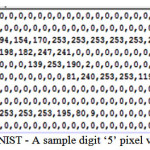
In the proposed method, an ANN has been implemented. First it is trained using back propagation. In the second case, deep belief nets have been used in which the network is first trained using deep learning and then refined using back propagation. MNIST database of handwritten digits has been used   for testing the network. MNIST database is a dataset available online which consists of 60,000 training examples to help train the model and 10,000 test examples from different areas which can be tested for checking accuracy. Each handwritten digit image is composed of 28*28 = 784 pixels. Fig 2 shows a very simple representation of pixel values for a sample digit ‘5’. (All pixels are not represented due to space constraints).

Figure 2: MNIST – A sample digit ‘5’ pixel values Click here to View figure

 

Pseudo code for Back Propagation

Create an ANN with n number of layers.

2. Initialize weights for all edges and biases for all nodes with small random numbers.

3. While terminating condition is not satisfied

DO

i. For each item in training data set do    

call ‘feedforward’ function passing the training data item to forward the inputs through all the layers

compare the outputs of the outermost layer computed post feed forward with the expected outputs and calculate error.  Back propagate the errors upto the input layer by calling ‘backpropagate’ function

Update the weights of each edge by calling the ‘updateWeights’ function

Update the bias of each node by calling the ‘updateBias’ function

End For

End While

feedforward function

Inputs: item to be feed forwarded

Outputs: forwards the input calculating the inputs and outputs at each layer

Pseudo code

Assign the inputs of the first layer from the item input. For MNIST handwritten digit recognition there are 784 pixels with values ranging from 0 to 255.  Normalize each pixel value by dividing the same by 255. Assign the normalized pixel values to each of the 784 input nodes. 

Make the outputs of the input layer same as inputs. That is for each input layer node j set O_j=  I_j.,where O_j , I_j  are output and input of j^th no respectively.

For each hidden layer unit j with a previous layer i, where w_ij is the weight of edges from a node   in layer i to a node in layer j and bias_j is thebias value for node j.

Assign I_j = Σ_iw_ijO_i+ bias_j [11]

Set O_j = 1 / (1 + exp(-I_j)) [11]

For output layer unit j with a previous layer i call ‘softmax’ function.

End

Softmax function [15, 16]

Output: Calculate ate outputs for the output layer in terms of probability distribution.  For a particular input digit to the network, outputs show how much is the probability of that digit is digit 0, how much is 1 and so on

Algorithm

Initialize a variable sum = 0

for each node j of the output layer i.

sum = sum + exp(-I_j)) , where exp is the exponential function

End for

for each node j of the output layer

i. Set O_j = exp(I_j))/ sum

End

backpropagate function

Input: actual output of the training sample T _j

Algorithm

For each unit j in the output layer calculate the error Err_j as

i. Set Err_j= T_j – O_j  [11]  

End for

for each unit j in the hidden layer from the last to the first hidden layer

i. Set Errj = (1- Oj) * (1+Oj) * Σ _k     Err_jw_jk [11]   –         here k is the next highest layer

End for

updateweights function

Algorithm

For each weight wij in the neural network

i. set Δw_ij = (learningRate) Errj * Oj

ii. updatew_ijas :

w_ij= w_ij+ Δw_ij [7]

End for

updatebias function

Algorithm

for each bias bias_jin the neural network

set bias_j = (learningRate) Err_j

Update bias_jas:

bias_j= bias_j+ Δ bias_j 2.  End for

Pseudo Code for Deep Learning with RBMs

The basic structure for this also remains same as back propagation above except that in the Pre-training step each two consecutive layer staring from the first layer are processed by RBM processing

Algorithm

For each pair of consecutive layers in the Network do

call   ‘doRBMProcessing’    function

End for.

doRBM Processing function

Inputs: Layer X and Layer Y of the neural network to be performed by RBM Processing. It is assumed that initializations of weights of weights, biases and input layer have already been done as above.

Algorithm

While termination criteria is not satisfied do

For each unit j in the Layer Y

Assign  I_j = Σ_iw_ijI_i  + bias_j /* where i is a node of LayerX */

Set O_j = 1 / (1 + exp(-I_j) )

End For

For each unit j in the Layer X

Assign  I_j = Σ_iw_jiO_i + bias_j /* where i is a node of LayerY */

Set O_j = 1 / (1 + exp(-I_j) )

End For

Compare Layer X inputs with the actual inputs and calculate error with respect to    the original inputs, then back propagate the error and update weights and biases using the same logic as described in the case of normal back propagation.

End While

Results and Discussions

Each training digit from the training data sample is passed through the layer in the learning phase. Then each digit from the test data sample is tested. Network is made to learn for different number of epochs. One epoch implies that the network is tested with the entire dataset once. Then each digit from the test data set is tested and accuracy is calculated with following formula:

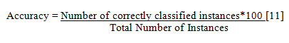
Table 1 and Table 2 show the observations for both the cases. Case I is where the network is first made to learn by simple back propagation algorithm and then tested. Deep learning has not been used in Case I. Case II is where deep learning has been used in the learning phase and then the network has been tested.

Table 1: Number of Epochs Vs Accuracy (Without Deep Learning)

Number of Epochs	Accuracy	Time Taken for Learning (ms)
1	89.05	1085307
2	90.12	1087391
3	92.79	1090120
4	93.34	1190210

 

Table 2: Number of Epochs Vs Accuracy (With Deep Learning)

Number of Epochs	Accuracy	Time Taken for Learning (ms)
1	92.39	2134123
2	92.35	2178901
3	93.29	2179210
4	94.12	2234405

 

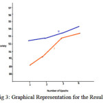
Fig 3 shows the graphical representation depicting the relation between the above two cases and depicts that accuracy increases with the number of epochs and is greater for case II then case I. On the negative side case II takes more time in learning than case I. So that can be made better by using parallel technologies such as Map Reduce.

Figure 3: Graphical Representation for the Results  Click here to View figure

 

Conclusion and Future Scope

An attempt has been made in this research to design and implement a basic deep belief network with a focus on improved accuracy. For this purpose the network has been successfully tested with MNIST images of handwritten digits. It has been concluded from the results that deep learning fine-tuned with back propagation shows a greater accuracy than when only back propagation is used alone. When the number of epochs are 1 and 2, an accuracy of about 2.785% is achieved with deep learning. For number of epochs as 3 and 4, this has been reduced to 0.34% which can be attributed to the fact to greater number of epochs and long training time involved in deep learning for training RBMs’. This can be extended in future to implement deep learning with distributed technologies such as Map Reduce to reduce the time involved .The solution implemented in this research is generic and can be tested for other such tasks also.

References

1. Bo Pang, Lillian Lee, and Shivakumar Vaithyanathan, “Thumbs up? sentiment classification using machine learning techniques”, in Proc. of the ACL-02 Conference on Empirical Methods in Natural Language Processing, vol. 10. ACM, Stroudsburg, PA, USA, pp. 79-86. DOI=http://dx.doi.org/10.3115/1118693.1118704.
   CrossRef
2. Hu, Minqing and Bing Liu. Mining and summarizing customer reviews. In Proceedings of ACM SIGKDD International Conference on Knowledge Discovery and Data Mining (KDD-2004).
   CrossRef
3. Syed Imtiyaz Hassan, “Designing a flexible system for automatic detection of categorical student sentiment polarity using machine learning”, International Journal of u- and e- Service, Science and Technology, vol. 10, issue.3, Mar 2017, ISSN: 2005-4246. (to be published in Mar 31, 2017)
4. Turney, P. Thumbs up or thumbs down?: semantic orientation applied to unsupervised classification of reviews. In Proceedings of Annual Meeting of the Association for Computational Linguistics (ACL- 2002).
5. MNIST handwritten digit database, YannLeCun, Corinna Cortes and Chris Burges”, Yann.lecun.com, 2016. [Online]. Available: http://yann.lecun.com/exdb/mnist/. [Accessed: 01- Dec- 2016].
6. G. Hinton and Y. Teh, A fast learning algorithm for deep belief nets, 1st ed. Toronto, 2006, pp. 1-5,8-11.
7. A. Chris Nicholson, “A Beginner’s Tutorial for Restricted Boltzmannn Machines – Deeplearning4j: Open-source, Distributed Deep Learning for the JVM”, Deeplearning4j.org, 2016. [Online]. Available: https://deeplearning4j.org/restrictedBoltzmannnmachine.html. [Accessed: 30- Nov- 2016].
8. Q. V. Le, A Tutorial on Deep Learning, 1st ed. Mountain View, 2015, pp. 10-15.
9. O.Matan ,Reading Handwritten Digits : A Zip Code Recognition System, 1st ed. Holmdel, 2016, pp. 5-15.
10. A Practical Guide to Training Restricted Boltzmannn Machines, 1st ed. Toronto, 2016, pp. 1-7.
11. J. Han and M. Kamber, Data Mining Concepts amd Techniques, 3rd ed. MA: Elsevier, 2012, pp. 398-407 ,327-332.
12. “Classification. Classification: predicts categorical class labels classifies data (constructs a model) based on the training set and the values (class. – ppt download”, Slideplayer.com, 2016. [Online]. Available: http://slideplayer.com/slide/5243492/. [Accessed: 01- Dec- 2016].
13. M. Mazue, “A Step by Step Backpropagation Example”, Matt Mazur, 2016. [Online]. Available: https://mattmazur.com/2015/03/17/a-step-by-step-backpropagation-example. [Accessed: 30- Nov- 2016].
14. “Training an Artificial Neural Network – Intro”, solver, 2016. [Online]. Available: http://www.solver.com/training-artificial-neural-network-intro. [Accessed: 30- Nov- 2016].
15. D. Yuret, “Softmax Classification — Knet.jl 0.7.2 documentation”, Knet.readthedocs.io, 2016. [Online]. Available: http://knet.readthedocs.io/en/latest/softmax.html. [Accessed: 01- Dec- 2016].
16. S. Raschka, “What-is-the-intuition-behind-SoftMax-function”, Quora, 2014. [Online]. Available: https://www.quora.com/What-is-the-intuition-behind-SoftMax-function. [Accessed: 01- Dec- 2016].
17. K. ZHANG and X. CHEN, Large-Scale Deep Belief Nets With MapReduce, 1st ed. Detroit: IEEE, 2014, pp. 1-5.
18. Syed Imtiyaz Hassan,  “Extracting the sentiment score of customer review from unstructured big data using Map Reduce algorithm”,  International Journal of Database Theory and Application, vol. 9, issue 12, Dec 2016, pp. 289-298doi:10.14257/ijdta.2016.9.12.26, ISSN: 2005-4270.
    CrossRef

---

This work is licensed under a Creative Commons Attribution 4.0 International License.