Training Neural Network Elements Created From Long Shot Term Memory

Kostantin P. Nikolic

Faculty of Management, Department of Informatics, Novi Sad

DOI : http://dx.doi.org/10.13005/ojcst/10.01.01

ABSTRACT:

This paper presents the application of stochastic search algorithms to train artificial neural networks. Methodology approaches in the work created primarily to provide training complex recurrent neural networks. It is known that training recurrent networks is more complex than the type of training feedforward neural networks. Through simulation of recurrent networks is realized propagation signal from input to output and training process achieves a stochastic search in the space of parameters. The performance of this type of algorithm is superior to most of the training algorithms, which are based on the concept of gradient. The efficiency of these algorithms is demonstrated in the training network created from units that are characterized by long term and long shot term memory of networks. The presented methology is effective and relative simple.

KEYWORDS: Artificial Neural Networks (ANN); Feed-forward Neural Networks (FNN); Recurent Neural Networks (RNN); Simulation Graph Model (SGM) networks; Stochastic Direct Search (SDS); Long Term Memory(LTM); Long Shot Term Memory (LST) units

Copy the following to cite this article: Nikolic K. P. Training Neural Network Elements Created From Long Shot Term Memory. Orient.J. Comp. Sci. and Technol;10(1)

Copy the following to cite this URL: Nikolic K. P. Training Neural Network Elements Created From Long Shot Term Memory. Orient.J. Comp. Sci. and Technol;10(1). Available from: http://www.computerscijournal.org/?p=4783

Introduction

An artificial neuron (ANe) is a simplified model of biological neurons (BNe) characteristic of the kind of relatively higher levels of development of life. The artificial neural network (ANN) is structured from the ANe’s. Since the method for creating term structure depends on the type of network ie. classification networks. We discuss the two types of networks according to the mode propagation through the ANN. ANN in which the signals are spread progressively advance from the entrance to the exit in the literature identified as FNN network¹. ANN in which there is at least one loop in the propagation of signals are called recurrent neural network (RNN)^1,2.  FNN network because of its specific characteristics is widely used. In the literature are represented almost 95% of the amount when compared to the RNN³. The reason for this are the problems of training and therefore create architecture RNN. Overcoming these problems is usually achieved by transformation into an appropriate RNN to FNN network. In this way, a precondition for the application of the algorithm back propagation (BP)⁴, but with some modifications, and when it was known as ‘BP over time’ ie BPTT⁵. Realization BPTT algorithm is much more complex than the standard BP⁶. Recurrent Back Propagation(RBP) is a method that does not use the transformation of the RNN to FNN but it starts so from the gradient of cost function¹⁸. The paper takes into account the training ANN with supervision. This type of training is very often used although it is not easy to deploy⁶. RNN type of network is very present in the neural structures of living things⁷ . This is one of the challenges for researchers, and the second is the complexity of performance that can be achieved with RNN networks. Appropriate architecture RNN can simulate the behavior of finite automata, including the Turing machine and Von Neumann’s universal programming automata that is modern computational machine⁸. Last implies greater application RNN network to recognize natural speech, recognize complex patterns and scripts⁸. RNN also its dynamics can simulate the behavior of dynamic systems with control^3,9 .Dinamic control systems are generally  realized of the  RNN with neurons type additive i.e. dynamic type of neurons¹⁰. Last is the reason for creating this work. The presented methodology enables training and synthesis of complex architecture RNN made of LTM and LST neurons as components.

Method

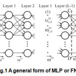
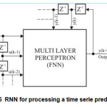
Recurrent neural network architectures can have many different forms. One common type consists of a standard Multy-Layer Perceptron (MLP) ie FNN on Fig.1, plus added loops.

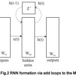
If the FNN on Fig. 1 split straight lines AB and CD, which represents intermittently, receives the same block depiction according to Fig.2.

Figure 1: A general form of MLP or FNN   Click here to View figure

 

Figure 2: RNN formation via add loops to the MLP  Click here to View figure

 

At the same block structure is added loop in which the unit delay(z^-1). In Fig. 2 behind the add feedback loop obtained is determined RNN. Functioning of this structure is mathematicaly described following terms:

h(t) = g_h(W_ih x(t)+W_hh h(t-1))                                (1)          

y(t) = g₀(W_h0 h(t))                  (2)                          

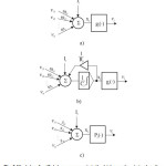
These can exploit the powerful non-linear mapping capabilities of the MLP, and also have some form of memory. Others have more uniform structures, potentially with every neuron connected to all the others, and may also have stochastic activation functions or synapses ¹¹(Fig.3, c).

The processing unit of which ANN is RNN can be made, as in the Fig.3 represents. The presence of certain neurons-perceptron can be monolithic or mixed. For imitation of technical control system using RNN most appropriate to use a monolithic structure type b) on  Fig.3.

Figure 3: Models of artficial neurons:  a)static, b)dynamic, c)stochastics    Click here to View figure

 

Such networks can be completely or incompletely related, which depends on the usage. Mathematical description of this relationship within the neural network is reduced to a certain set of differential equations of the first order¹³.

For the connection of any two of the RNN perceptron network, can be set equations:

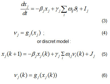
where  :  x_j – activation potential of j-th perceptron,

ω_ij – synapse (weight) that connects the observed perceptrons i and j,

v_j – ouput of the j-th internal perceptron and v_i intputs from internal  i– perceptron,

g_j –  is activaton function of j-perceptron,

I_j – represents bias j-th perceptron (ω_oj),

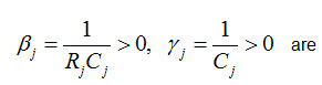
are appropriate constants.

The relations (1), (2) so  can be rearranged and displayed via the discretized time t with step Δt=1:

h(k)=g_h(W_ih x(k)+W_hh h (k-1))                              (7)

y(k+1)=g₀(W_h0 h(k))                                             (8)

where  W_ih, W_hh, W_h0  are matrixs of coresponding synapsis (Fig.2) .

If ascended into account that the MLP i.e. FNN in the Fig.1 and Fig.2 be added to the feedback branches, not only the delay units but neurons or groups of neurons presented at Fig.3 a) and b), then the relation (7) and (8), with introduction W_back can rearrange to form:

x(k+1)=g(W_ihu(k+1)+W_hhx(k)+W_backy(k ))                 (9) 

y(k+1)=g_o(W_o(u(k+1), x(k+1))                                    (10)

where x(k+1) is actvation of internal units,y(k+1) output, u(k) is vector of input units, u(k+1) extrernally inputs, x(k) internal  inputs with an aktivation vector, y(k) output vektor;   all matrix  in expressions (9) and (10) are  certain dimensions composed of values ω_ij synapses between appropriate perceptrons  i and j; g and g₀ are aktvation functions sigmoidal type; (u(k+1), x(k+1)) denotes the contatenated vector made of input and actiation vectors.

To monitoring the behavior of neural network training with the benefits of an error at the output of the system:

e(k)=y(k) – y^tp(k); tp-denotes training pair,                                                    (11)

or function criteria(cost function):

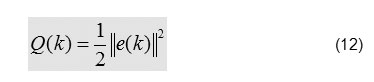
Most methods use the term gradient of Q(k) i.e Grad( Q (k)).

The best known methods of standard BP and BPTT use the following multi-step algorithm for optimization and training^4,5 :

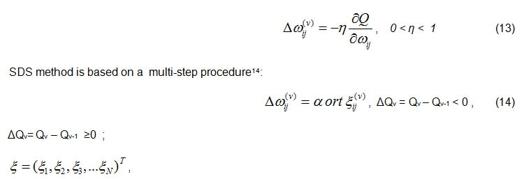
where ξ random variable uniform distribution; for Δ Q <0 there is a successful step(v) until search for ΔQ ≥0 unsuccessful; α  is coefficient learning speed (0<α<1), T-denotes transpose, N-denotes number of synapses ω_ij  i.e. all parameters in network( ω_ij , β_j, ɣ_j).

SDS algorithm is defined as above is able-bodied but without additional heuristics is not effective in practice. Algorithm MN-SDS has some heuristics that makes it effective. The basic definition of MN-SDS algorithm¹⁵  is given with:

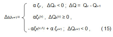
where:  ζ_v = ort ξ_v ;  ζ_v – is refered to v  step of iterration,  ∆Q_v – increment of cost function  Q  in ν  effective iteration step;  ζ_R^(v,Λ),  αζ_R^(v,Λ) – is resultant  of all failed steps ζ_λ^(v) ,∆Q_λ^(λ)–  increment of Q for failed steps λ,  λ=1,2,3,…,Λ; ζ_v+1 is first step with Δ Q _v+1<0 after λ=Λ ; for ξ  and  ζ to apply the relation  |ξ|≤1,  |ζ|=1; 0< α < 1.

The using ortξ=ζ is nessesary for the improvement stability of process training. Minimum of  a cost function Q is obtained in forward stage.without forward back propagation steps.  This is one of the advantages of SDS.

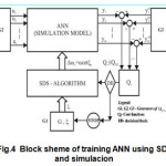
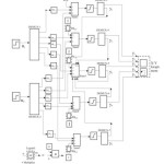
For the successful implementation of SDS i.e. MN-SDS on the training of ‘Real-Time RNN’ (RTRNN) it is necessary to time discretization of the process in the network and simulation model of graph presentation network ( Fig.4).

Because of the difficulties that exist in mathematical numerical simple procedures both for signal propagation and the minimization criterion function, the paper goes simultaneously with the simulation and implementation of SDS RNN algorithms.

Figure 4: Block sheme of training ANN using SDS and simulacion Click here to View figure

 

So, behind the transformation of RNN to a corresponding simulation model network optimization i.e. training is delivered through the simulation model. This scheme is presented on Fig.4.  Between the simulation model and the network RNN there is correspondence appropriate entities. The scheme (Fig.4) contains the auxiliary devices for automatic optimization of procedure of training ie: random number generator G1, generators G2 and G3 training pairs with a sinhronisation possibility, and  a decision block DB for the completion of certain procedures.  The presented methodology can be characterized as a blackbox method¹⁶

In the simulation model of the network can be monitored propagation signal from input to output without any numerical procedure. Also a selection of a certain scaling of the process creates additional comfort for a successful procedure of training.The success of this approach largely depends on the software packages for a simulation.

This approach can be applied to training ANN i.e. RNN network considerable complexity. For the case of RNN and RTRNN this represents a challenge for researchers and designers.

Results

Each methodology is built to solve a specific problem or a specific set of problems. Working ability of the method lies in the facilitation of its applicability to its effectiveness takes for an acceptable interval of time and that its exploitation acceptable by price. SDS methods, according to all the above requirements ahead of BP and BPTT method. To a certain extent, this can be said of method of training “Recurenta Back-Propagation” (RBP)¹¹. Of all  these frequently used methods of training neural networks, SDS is characterized by simple heuristic logic and numerical procedures. Important is the fact that SDS method characterized by better convergence¹⁴. Also grows the more complexity to the network edge, which is linked to convergence, the increasing in favor SDS method ^14,15. Simulation only increases the benefits of SDS above mentioned methods.

The method that is presented in performance over the SDS methodology is Kalmann Extended Filtering (EKF)¹⁷. This is understandable when we take into account the dynamics of networks such as RNN. However, it must be emphasized that a number of math- transformation and  also use the partial differentiation in certain stages of the method, generates a lot of trouble. SDS method because of its mathematical-logical simplicity to some extent deprived of these problems¹⁴.

Let us mention the fact that the SDS algorithm MN-SDS possesses the ability of self-learning so it is very flexible, especially in the case of high complexity RNN network dimensions through 100th.  MN-SDS algorithm works well, and in this case: it is not too sensitive to the suspect can be applied when all other parameters are changing. In large network complexity to the application MN-SDS algorithm in the training of network systems react similarly with the property of homeostasis. Previously leads to the conclusion that a stable network at a metered shift parameters and remain stable .

To gain insight into the procedure of applying the methodology are examples of relatively simple RNN Networks.

Example-1

In this case points to the simple construction and the MLP unit delay (Fig.5), which plays an important role in signal processing i.e. processing time series signals. It is very common in applying for prediction and forecasting.

Figure 5: RNN for processing a time serie prediction  Click here to View figure

 

This type of network considered by many important species NARX RNN neural network. If the input vector u defined as :

u = [u (k-1), u (k-2), …, u(k-p)]^T,                    

then p is called a predictor of the first order¹⁸; scalar value MLP output is y = ύ(k); actual y(k) is the desired respond, u(k)-ύ(k)=e’(k) is the error of approximation u(k); T-denotes transpose.

How to apply RNN relations (9) and (10) it follows that there is a relation: u (k + 1) = y (k + 1) If we bear in mind how this works RNN appears that the network will have a prediction for the value of u(k).

Example-2

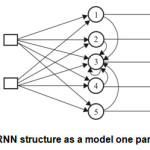
Neuro-structures in the central nervous system (CNS)  are usually recurrent biological neural networks. Model neuro-structure that performs the modification state of excitation and inhibition depending on the level value of the input signal and thus changes the innervation of certain of functional neural structures⁷ , is shown in Fig.6.

Figure 6: RNN structure as a model one part of brain    Click here to View figure

 

Figure 7: Simulation model  RNN with image Fig.6  Click here to View figure

 

The simplicity of the model RNN network has taken to demonstrate the transition from the graph model of the network at an appropriate simulation model (Fig.7). Behind the creation of symbolic simulation model of the rest of the grid is implemented via software modules selected software package¹⁹

Discussion

Advantages SDS algorithms to train ANN static type FNN with some changes heuristics are transmitted with a network of training RNN. In this paper, the introduction of a simulation model ANN extended application SDS algorithms for training not only RNN but RTRNN networks. In accordance with the foregoing SDS algorithms can successfully be applied at ANN, which includes LST building units. This makes them suitable both in research projects   so in engineering practice. ^. Creating significantly more complex architecture of the RNN, than with the Fig.6, (which can usefully to use for the recognition of natural speech, handwriting, etc) it can to achieve across the copied analog structures of the central nervous system of human brain. In this procedure can help a lot functional magnetic resonance imaging^20,21.

Conclusion

This paper presents the application of stochastic search algorithms to train recurrent artificial neural networks. Methodology approaches in the work created primarily to provide training complex recurrent neural networks. It is known that training recurrent networks is more complex than the type of training feed-forward neural networks. The introduction of a simulation model of the neural network and discretization of continuous signals, overcome the disadvantages of SDS algorithms have when it comes to training ANN with dynamics. Through simulation of recurrent networks is realized propagation signal from input to output automatically without any additional numerical procedures. Training per pair realized iterative steps shift parameters using SDS custom heuristic algorithms behind the self-study. Procedures training is a type of supervision The performance of this type of algorithm is superior to most of the training algorithms, which are based on the concept of gradient i.e. BP, BPTT and RBP. The efficiency of these algorithms is demonstrated in the training network created from units that are characterized by long term and  long shot term memory of networks. The main advantage of SDS algorithms is that they are achieving the best results in working with  ANN complex architectures. An important moment in the application of the methodology presented is the selection of a software package for the simulation. Valid results of numerical experiments are achieved by software package SIMULINK of The Math Works, 2015 b.

References

1. Haykin S.  Neural Networks, Macmilan College Publishing Company, New York,1994.
2. Metskar L.R. and Jain L.S.. Recurrent Neural Networks: Design and Applications. The CRS Press International Series on Computational Intelligence 2000.
3. Jeager H. A tutorial on training recurrent neural networks, covering BPTT, RTL, EKF and the “echo state network” approach. Fifth revision,  FraunhoverInstitute Autonomous Intelligent System (AIS); International University Bremen, 2013.
4. Rumelhart D.E., Hinton G.E. and Williams R.J.: Learning Representation by Back-propagation Errors. Nature, 1986a; No 232, pp 533-536.
   CrossRef
5. Rumelhart, D.E., G.E. Hinton, and R.J. Williams. Learning internal representations by error propagation. In Parallel Distributed Processing: Explorations in the Microstructure of Cognition. Vol. 1 Chapter 8, Cambridge, MA: MIT Press. 1986.
6. MilenkovicS.  Artficial Neural Networks. Doctoral Thesis,  Foudation Andrejevic, 1997, pp 40-44.
7. Shade J.P. and Ford D.H., Basic Neurology, Elsevier Scientific Publishing Company (Second Revised Edition), Amsterdam, London, New York, 1973
8. Siegelmann H.T. and Sontag E.D Computational Power of Recurrent Networks, Applied Mathematics Letters, 1991, Vol 4, pp 77-80
   CrossRef
9. Ku C.C. and  Lee K.Y., Diagonal Recurrent Networks for Dynamic Control. In IEEE Transaction of Neural Networks, Vol.6,N 1, 1995
10. Patrick S. and Krose B,  Robot Control, In Introduction to Neural Networks, Eghth edition, 1996, pp 85-95.
11. Haykin S.  Stochastic Neurons. In Neural Networks, Macmilan College Publishing Company, New York, 1994, pp 309-311..
12. Milenkovic S.,   Dynamic Models, In    Artficial Neural Networks. Doctoral Thesis,   Foudation Andrejevic, 1997, pp 19-22
13. Pineda F.J., Generalization of  Back- Propagation to Rekurrent     Neural Networks, Phisical Review Letters, vol 59, N 19, 1989.
14. Rastrigin, L.A. Comparison of methods of gradient and stochastic search methods. In: Stochastic Search Methods., Science Publishing, 1968; Moscow, Russia. pp. 102-108
15. Nikolic K.P.: Stochastic Search Algorithms for Identification, Optimization and Training of Artificial Neural Networks. International Journal AANS, Hindawi, 2015
16. Hemsoth N.  Black Box Problem closes in on Neural Networks, Wikipedia, 2015
17. Feldkamp L.A., Prokhorov D., Eagen C.F. and  Yuan F., Enhanced multi–stream Kalman filter training for recurrent neural networks. In X XX (ed.) Nonlinear modeling advanced black –box techniques, 1986, Boston Kluwer, pp 29-53.
18. Haykin S., Recurrent Beak-Propagation, In Neural Networks, Macmilan College Publishing Company, New York, 1994, pp 577-588.
19. SIMULINK of MATLAB 2014b, The MATH WORKS Inc, 2014.
20. Sporns O. Networks of the brain.  The MIT Press. Cembridgs, Massachusetts, London, England, 2011.
21. Sporns O., Discovering the human connectome. The MIT Press. 2012.

---

This work is licensed under a Creative Commons Attribution 4.0 International License.