Prediction of Bike Sharing Demand

Purnima Sachdeva and K N Sarvanan

Department of Computer Science, Christ University, Bangalore, 560034, India

 

E-mail: saravanan.kn@christuniversity.in

 

DOI : http://dx.doi.org/10.13005/ojcst/10.01.30

ABSTRACT:

Bike sharing systems have been gaining prominence all over the world with more than 500 successful systems being deployed in major cities like New York, Washington, London. With an increasing awareness of the harms of fossil based mean of transportation, problems of traffic congestion in cities and increasing health consciousness in urban areas, citizens are adopting bike sharing systems with zest. Even developing countries like India are adopting the trend with a bike sharing system in the pipeline for Karnataka. This paper tackles the problem of predicting the number of bikes which will be rented at any given hour in a given city, henceforth referred to as the problem of ‘Bike Sharing Demand’. In this vein, this paper investigates the efficacy of standard machine learning techniques namely SVM, Regression, Random Forests, Boosting by implementing and analyzing their performance with respect to each other.This paper also presents two novel methods, Linear Combination and Discriminating Linear Combination, for the ‘Bike Sharing Demand’ problem which supersede the aforementioned techniques as good estimates in the real world.

KEYWORDS: Learning; Neural Networks; Random Forests; Regression; SVM; Gradient Boosting; Boost; Linear Combination; Python; Weak Learner; Strong Learner.10

Copy the following to cite this article: Sachdeva P, Sarvanan K. N. Prediction of Bike Sharing Demand. Orient.J. Comp. Sci. and Technol;10(1)

Copy the following to cite this URL: Sachdeva P, Sarvanan K. N. Prediction of Bike Sharing Demand. Orient.J. Comp. Sci. and Technol;10(1). Available from: http://www.computerscijournal.org/?p=4937

Introduction

Bike sharing systems are innovative ways of renting bicycles for use without the onus of ownership . A pay  per use system,  the bike  sharing model is either  works in two modes: users  can get  a membership  for cheaper rates  or   they can  pay for the bicycles  on an ad-hoc basis. The  users of bike sharing systems can pick up bicycles from a kiosk in one location and return them to a kiosk in possibly any location of the city.

Bike sharing systems have been gaining a lot of traction around the world [1] and feasibility studies are being taken up all over the world like Australia [13], Sao Paulo [14], China [15] to understand the infrastructural requirements as well as the benefits and impact of the same on the citizens. With more than 500 bike renting schemes across the globe, and popular bike renting programs functional in London (Boris bikes), Washington (Capital bikeshare) and New York (Citi bikes) which are used by millions of citizens every month; these schemes provide rich dataset for analysis. This prompted the authors of this paper to take up the interesting problem of inventory management [16] in bike sharing system, which can be formulated as the ‘Bike sharing demand’ problem wherein given a supervised set of data, you have to create a model to predict the number of bikes that will be rented at any given hour in the future.

Table 1:  Variables In The Dataset

Variable	Type	Remarks
datetime	Datetime
season	Integer	1(Spring), 2(Summer), 3(Fall), 4(Winter)
holiday	Boolean	1(Holiday)
working day	Boolean	1(Working Day)
weather	Integer	1(Clear), 2(Mist), 3(Snow), 4(Heavy Rain)
temp	Decimal	degrees Celsius
atemp	Decimal	apparent temperature in degree Celsius
humidity	Integer	relative humidity percentage
windspeed	Decimal	speed of air
casual	Integer	number of non-registered bike shares in the hour
registered	Integer	number of registered bike shares in the hour
count	Integer	total number of bike shares in the horu

 

The data generated by these systems can be analyzed to

Figure 1: Correlation Matrix of all feature variables  Click here to View figure

 

draw inferences regarding market forces which in this particular case translates to bike sharing demand. Factors such as time and duration of travel, season of renting, temperature etc, play an important role in determining the patterns of bikes renting demand in a city. While this paper uses data from the Capital Bikeshare program in Washington, D.C., to come up with a model, the results can be generalized to any city with minimal effort by retraining the models.

The conclusions in this project are drawn from various models which were implemented and tests to predict the bike sharing demand for the provided dataset. In particular, two presented models Linear Combination and Discriminating Linear Combination proved to be reasonably efficient in predicting the demand and ranked in the top 1% of Kaggle.

The rest of this report is organized as follows: Section II is an overview of the dataset, Section II-A explains the major feature engineering employed, Section II is an overview of the different models implemented and Section IV lays down the results of the experiments.

Data 

The dataset in this project is provided by Kaggle and is an open dataset hosted at UCI Machine Learning Repository[2] on behalf of Hadi Fanaee Tork. The data includes rental and usage data of bike renting spread across two years and is described in Table I.

The trading data has 10866 observations of 12 variables, while the test data has 6493 observations of 9 variables. The training set consist of rental data for the first two-thirds of each month, while testing data comprises of the remaining third.

Feature Selection

To make the data tenable for understanding and further analysis , the data set was analyzed for identifiable statistical trends and patterns. After preliminary analysis, the following steps were undertaken to transform the data into a systematically workable dataset:

• Changing date-time into timestamps
• Splitting timestamps into days, months, years and day of the week.
• Converting season, holiday, working day and weather into categoric variables or factors.
• Converting hours into a factor.

These transformations allowed us to extract certain key features of the dataset namely, the day of the week and the year, which proved to be pertinent in further analysis.

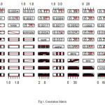
To refine the data further, a correlation matrix was created amongst all the feature variables to analyze interaction effects. Figure II-A shows the correlation matrix thus obtained and the patterns observed. Analysis of the correlation matrix revealed the following salient points:

• temp and atemp were highly correlated with a pearson correlation coefficient greater than 0.98.
• month and season also had a high pearson correlation coefficient of 0.97.

Figure 2: Feature importance graph of Random Forest   Click here to View figure

 

Ipso facto, month and atemp were removed from the universe of features to avoid overfitting and redundancies.

Method

Prima Facie, a number of standard [3] machine learning techniques were implemented on the data:

• SVM [4] with different kernels [5]
• Neural Network [6]
• Poisson Regression

The lackluster performance of these methods was attributed to several reasons. Neural networks work best on data with continuous variables, in contrast to the dataset for this particular problem which consists mostly of categorical variables. The performance also motivated the use of more sophisticated machine learning models, namely Random Forests and Gradient Boosting which has been discussed in the subsequent subsections:

Random Forests

Random Forests [7] work by creating multiple weak learners for different subsets of the training set which are then combined to form a strong learner. The fundamental idea underlying Random Forests is that training a decision tree repeatedly on a dataset produces a new decision tree every time and multiple such trees reduce the overall error of the model.

The decision of using Random Forests was driven considering the weak performance of Neural Networks on the dataset, which was expected considering that the problem is not amenable to them.

The experiments were carried out in Python using scikit-learn’s ensemble Random Forest classifier. In order to tune the parameters for the model, scikit-learn’s excellent GridSearchCV was employed which performs an  exhaustive search on the different parameters of Random Forest, using cross validation to find an optimum value for each of the parameters. The parameters under consideration that were tuned using GridSearchCV were as follows:

• number of estimators: which are the number of trees in a Forest
• max number of features: the number of features considered to split on at each node

The optimal parameters discovered using this method turned out to be a total of 100 estimators and the max number of features to split on at each node was 3. Learning a Random Forest model on the data then reduced the RMSE (Root Mean Squared Logarithmic Error) [10] from 0.46 for Neural Networks to 0.39 which was a marked improvement in performance.

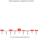
A way to analyse the relative effectiveness of Random Forests is to study the feature importance graph (Figure 2). The graph obtained for our particular model was heavily skewed towards the ‘hour’ variable, with little to no importance being assigned to the other variables in the dataset. Which does not paint a rosy picture for the model as a whole.

In an attempt to rectify this skewed feature importance and increase the performance of Random Forests, a variant of the model knows and Extra Trees Regressor [8] (which performs random splits at a node level on the tree) was used. The change in RMSE for the two models was not significant enough to merit considering Extra Trees Regressor as a better model than Random Forests and prompted us to take us more sophisticated models for the problem at hand.

• Learning rate: the importance given to error residuals at every iteration
• Max Depth: maximum depth of each tree
• Minimum samples in the leaf: the minimum number of samples in each leaf node.

Gradient Boosting

Gradient Boosting [9] like Random Forests is an ensemble learning method. Similar to latter, it uses multiple weak learners which are combined to form a strong learner. But unlike its Random Forests, Gradient Boosting as the name suggests uses boosting.

Boosting methods work iteratively to create a new learner at every stage; these new learners are then trained on the error residuals at a current iteration to produce new learners which are stronger than the previous stage. Applied to decision trees, every decision tree is works on the error residuals of the previous iteration to produce a better decision tree. The collection of these decision trees is then used as the overall model for predicting values.

The analysis was carried out in python using scikit-learn’s Gradient Boosting ensemble learning methods. In order to tune the parameters for the model, we took a feather from the original Gradient Boosting paper [9] which suggests tuning other parameters by first keeping the number of estimators very high and then obtaining the number of estimators using these optimal parameters.

Akin to the methods employed for Random Forests, we used GridSearchCV from scikit-learn to find an optimum setting for the following parameters:

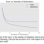
The optimum parameters found in the first iteration were 0.4 for learning rate, 3 for max depth and 15 for minimum samples in leaf, with the number of estimators fixed at 500. In the second stage of parameter estimation, the dependence of error of the model vs number of estimators used (Figure 3) was plotted for a validation set. The elbow of error – where the error plateaus off – on the validation set on the graph was used as the number of estimators, which turned out to be 85 for the given dataset

Figure 3: Feature importance graph of Gradient Boosting   Click here to View figure

 

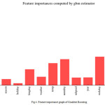Figure 4: Plot of the error vs the number of estimators used in predicting for Gradient Boosting. (The plot has an elbow at 85 with respect to the number of estimators used)   Click here to View figure

 

Gradient Boost outperformed Random Forest by a slight margin 0f 0.02 with a RMSE error of 0.37. Analyzing the feature importance graph of the used Gradient Boosting model in Figure 4 showed a more even distribution of importance across the different variables compared to Random Forests (Figure 2) even though the model was still skewed towards the ‘hour’ variable, which shows the importance of the time of day in predicting the overall demand.

Figure 5: Bimodal distribution of hourly frequency   Click here to View figure

 

Linear Combination

The difference in performance and feature importance of Gradient Boosting in Figure 4 and Random Forest in Figure 2, points to a different underlying structure of the data learned by each model which can be combined to produce a stronger model to represent it.

A simple linear combination of the two models weighted by their relative performance on a validation set was used to verify this hypothesis. (the weights so obtained were 0.6 for Gradient Boosting model and 0.4 for Random Forest model). This new linear combination model outperformed all tested models with an RMSE of 0.368.

Discriminating Linear Combination

Utilize information in the data regarding two distinct kinds of users: casual and registered as indicated in Table I, suggest a natural method of dividing the data into two logical groups for further analysis.

By applying the Linear Combination model separately for each of the two partitions of the data and adding the results for each partition (by virtue of the two partitions being mutually exclusive and exhaustive, we can simply add up the predicted results to get the final result) we obtain a new model – Discriminating Linear Combination. This model could be used to effectively understand the importance of memberships in bike sharing systems.

The performance of Discriminating Linear Combination was at par with Linear Combination model in terms ofRMSE which repudiated the hypothesis that memberships present additional information about the underlying data.

Table 2: Performance of Models in RMSE

Model	RMSE
SVM	0.43
Neural Network	0.46
Poisson Regression	0.42
Random Forest	0.39
Extra Trees Regressor	0.39
GBM	0.37
Linear Combination Model	0.36
Discriminating Linear Combination Model	0.36

 

Hour Sliced Model

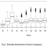
The feature importance graphs of Random Forests (Figure 2) and Gradient Boosting (Figure 4) show the importance of the time of day in predicting the demand of bike sharing at any given hour. In order to dissect this trend, a boxplot of bike rentals per hours (or the frequency distribution of number of rides taken at any given hour) was plotted.

This obtained distribution is a lower dimensional projection of the twelve dimensional feature vector and has two modes (hours when the bikes rented drastically increased). The modes of this bimodal distribution correspond to 8am and 5pm buckets.

A qualitative understanding of this trend can be set out as these modes correspond to times when working citizens go to and come back from their offices respectively; they are also the times when students go to and come back from their schools or colleges respectively which results in these marked increase in demand.

In an attempt to quantify this trend, the data was divided into four buckets, six hours each to create a new categoric variable called ‘time of day’. We then trained our proposed models on this new dataset but to no avail as both models failed to report any significant improvements when using this new dataset (it stands to reason that this might be because of the high correlation between hour and ‘time of day’ features, but removing the former did not lead to any significant result). 

Results

Table II lists down the performance of the various models written about in the previous sections in terms of their Root Mean Square Logarithmic Error (RMSE). In case of RMSE, lower values correspond to better models. As indicated in the table, our proposed Linear Combination model and Discriminating Linear Combination models outperform other models.

Conclusions

The experiments demonstrated in this paper reveal that Linear Combination model and Discriminating Linear Combination model are good models for predicting bike sharing demand with RMSe being close to 0.36.

Using the proposed models of Linear Combination and Discriminating Linear Combination, places us in the top 40 ranks of Kaggle’s bike sharing demand competition or top 1% percentile without accounting for falsified ranks in the competition which provides a reasonable benchmark for evaluating the efficacy of the models.

Future Work

The work carried out in this paper indicates that future work can be taken up in better representing the data and its underlying structure using state of the art techniques. Future work includes exploring more methods for feature engineering like splitting the data on the basis of working day and non working day and then training two separate models, or using hourly frequencies for different features in the data to extract more information as pursued in the Hour Sliced Model.

 Statistical methods like sampling should be used to handle the unbalanced nature of data with respect to a couple of categorical variable such as weather (very few instances of heavy rainfall are present in the dataset). Additionally random sampling can be used to create the training and test data set as the current framework of taking the first two-thirds of the month for the training set and last third for training set could induce some systematic bias in the model.

Dimensionality reduction techniques [11] like Principal Component Analysis [12] can also be employed to expose the underlying structure of the dataset, and re-evaluate the individual models listed in this paper to better understand the models.

Acknowledgment

We would like to thank Christ University for providing up the apparatus and facilities to carry out research and experimentation which made us pursue this problem with unbridled zest.

We would also like to thank our parents who have been with us through thick and thin and our guides at Christ University who have been instrumental in showing us the right direction.

Lastly, we would like to acknowledge our friends who are too many to mention in this small section but have helped us in small but meaningful ways like proofreading the paper for grammatical errors or inconsistencies.

References

1. Shaheen, Susan, Stacey Guzman, and Hua Zhang. ”Bikesharing in Europe, the Americas, and Asia: past, present, and future.” Transportation Research Record: Journal of the Transportation Research Board 2143 (2010): 159-167
   CrossRef
2. https://archive.ics.uci.edu/ml/datasets/Bike+Sharing+Dataset
3. Kotsiantis, Sotiris B., I. Zaharakis, and P. Pintelas. ”Supervised machine learning: A review of classification techniques.” (2007): 3-24.
4. Corinna Cortes and Vladimir Vapnik. Support-vector networks. Machine learning,20(3):273297, 1995.
   CrossRef
5. Scholkopf, Bernhard, and Alexander J. Smola. Learning with kernels:support vector machines, regularization, optimization, and beyond. MIT press, 2001.
6. Funahashi, Ken-Ichi. ”On the approximate realization of continuous mappings by neural networks.” Neural networks 2.3 (1989): 183-192.
   CrossRef
7. Leo Breiman. Random forests. Machine learning, 45(1):532, 2001.
   CrossRef
8. Geurts, Pierre, Damien Ernst, and Louis Wehenkel. ”Extremely randomized trees.” Machine learning 63.1 (2006): 3-42.
   CrossRef
9. Jerome H Friedman. Stochastic gradient boosting. Computational Statistics and Data Analysis, 38(4):367378, 2002.
10. Armstrong, J. Scott, and Fred Collopy. ”Error measures for generalizing about forecasting methods: Empirical comparisons.” International journal of forecasting 8.1 (1992): 69-80.
    CrossRef
11. Fodor, Imola K. ”A survey of dimension reduction techniques.” Center for Applied Scientific Computing, Lawrence Livermore National Laboratory 9 (2002): 1-18
    CrossRef
12. Jolliffe, Ian. Principal component analysis. John Wiley and Sons, Ltd, 2002.
13. Somers, A., and H. Eldaly. “Is Australia ready for Mobility as a Service?.” ARRB Conference, 27th, 2016, Melbourne, Victoria, Australia. 2016.
14. Verbruggen, K. J. P. Shared cycling infrastructure as a feeder system for public transport in Sao Paulo. BS thesis. University of Twente, 2017.
15. Chen, Mengwei, et al. “Public Bicycle Service Evaluation from Users’ Perspective: Case Study of Hangzhou, China.” Transportation Research Board 96th Annual Meeting. No. 17-04234. 2017.
    CrossRef
16. Raviv, Tal, and Ofer Kolka. “Optimal inventory management of a bike-sharing station.” IIE Transactions 45.10 (2013): 1077-1093.
    CrossRef

---

This work is licensed under a Creative Commons Attribution 4.0 International License.