Constructive and Clustering Methods to Solve Capacitated Vehicle Routing Problem

M. A. H. Akhand^* , Tanzima Sultana, M. I. R. Shuvo and Al-Mahmud

Dept. of Computer Science and Engineering Khulna University of Engineering and Technology (KUET) Khulna-9203, Bangladesh.

Corresponding author Email: akhandkuet@yahoo.com

DOI : http://dx.doi.org/10.13005/ojcst/10.03.02

ABSTRACT:

Vehicle Routing Problem (VRP) is a real life constraint satisfaction problem to find minimal travel distances of vehicles to serve customers. Capacitated VRP (CVRP) is the simplest form of VRP considering vehicle capacity constraint. Constructive and clustering are the two popular approaches to solve CVRP. A constructive approach creates routes and attempts to minimize the cost at the same time. Clarke and Wright’s Savings algorithm is a popular constructive method based on savings heuristic. On the other hand, a clustering based method first assigns nodes into vehicle wise cluster and then generates route for each vehicle. Sweep algorithm and its variants and Fisher and Jaikumar algorithm are popular among clustering methods. Route generation is a traveling salesman problem (TSP) and any TSP optimization method is useful for this purpose. In this study, popular constructive and clustering methods are studied, implemented and compared outcomes in solving a suite of benchmark CVRPs. For route optimization, Genetic Algorithm (GA), Ant Colony Optimization (ACO) and Velocity Tentative Particle Swarm Optimization (VTPSO) are employed in this study which are popular nature inspired optimization techniques for solving TSP. Experimental results revealed that parallel Savings is better than series Savings in constructive method. On the other hand, Sweep Reference Point using every stop (SRE) is the best among clustering based techniques.

KEYWORDS: Ant Colony Optimization; Capacitated Vehicle Routing Problem; Constructive method; Clustering method; Clarke and Wright’s Savings Algorithm; Fisher and Jaikumar Algorithm; Genetic Algorithm; Sweep Algorithm; Velocity Tentative Particle Swarm Optimization

Copy the following to cite this article: Akhand M. A. H, Sultana T, Shuvo M. I. R, Al-Mahmud. Constructive and Clustering Methods to Solve Capacitated Vehicle Routing Problem. Orient.J. Comp. Sci. and Technol;10(3)

Copy the following to cite this URL: Akhand M. A. H, Sultana T, Shuvo M. I. R, Al-Mahmud. Constructive and Clustering Methods to Solve Capacitated Vehicle Routing Problem. Orient. J. Comp. Sci. and Technol;10(3). Available from: http://www.computerscijournal.org/?p=6623

Introduction

Vehicle Routing Problem (VRP) is a real life constraint satisfaction problem to find minimal travel distances of vehicles to serve customers.¹ Capacitated VRP (CVRP) is the simplest form of VRP considering equal vehicle capacity constraint.² In CVRP, all customers have known demands and known locations for the delivery. The delivery for a customer cannot be split. In other words, the demand of a customer must be satisfied via only one visit. Goods are delivered from single depot and the vehicles return to the depot after serving their assigned customers. The delivery or unloading time may or may not be considered. The objective of CVRP is to minimize the total travelling distance for all vehicles.

Various ways have been investigated for solving the CVRP. Nearly all of them are heuristics because no exact algorithm can be guaranteed to find optimal tours within reasonable computing time when the problem is large. A heuristic approach does not explore the entire search space rather tries to find an optimal solution based on the available information of the problem. CVRP solving heuristic approaches are categorized as constructive and clustering methods. Constructive methods build a feasible solution gradually while keeping an eye on solution cost, but it may not contain an improvement or optimization phase. Some well-known algorithms of constructive methods are – Clarke and Wright’s Savings Algorithm.^3,4,5,6,7 Matching Based Algorithm and Multi-route Improvement Heuristics.⁸ On the other hand, clustering methods solve problem in two steps and that is why this approach is also called 2-phase or cluster first, route second method. First phase of this approach uses clustering algorithm to generate clusters of customers and second phase uses optimization technique to find optimum routes for each cluster generated in the first step. Sweep.^9,10 and Fisher and Jai kumar¹¹ are popular clustering algorithms.

This study investigates and compares performance of prominent constructive and clustering methods to solve CVRP and hence find out the best suited one. The initial clusters found from clustering methods are subjected to route optimization. For route optimization, Genetic Algorithm (GA).¹² Ant Colony Optimization (ACO)¹³ and Velocity Tentative Particle Swarm Optimization (VTPSO)_¹⁴ are employed in this study which are popular nature inspired optimization techniques for solving TSP. Though constructive methods generate optimal routes, route optimization techniques are also applied to Savings algorithm for performance analysis.

The outline of the paper is as follows; Section II explains prominent constructive and clustering methods briefly. Section III gives brief description of the optimization techniques. Section IV is for experimental studies in which outcomes of the selected methods are compared on a suite of benchmark CVRPs. At last, Section V gives a brief conclusion of the paper.

Constructive and Clustering Methods to Solve Cvrp

Constructive and clustering methods are popular in solving CVRPs. In this section prominent methods are explained briefly.

Constructive Method

A method in this category constructs routes as well as tries to minimize the traveled distance of the vehicles at the same time. Clarke and Wright’s Savings algorithm is the most popular constructive method and which is explained below.

Clarke and Wright’s Savings Algorithm

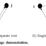
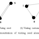
The algorithm is based on savings distance³ which is obtained by joining two routes into one route as illustrated in Fig. 1 where point 0 represents the depot. Denoting the transportation cost between two given points i and j, total transportation costs for separate (Fig. 1(a)) and single visit (Fig. 1(b)) are shown in Eq. (1) and Eq. (2), respectively.

D_a= C_0i+ C_i0 + C_{0 j} + C_j0                                   (1)

D_b= C_0i+ C_ij+ C_j0                                                 (2)

Now, the distance saved (savings distance) by visiting i and j in the same route instead of separately is,

S_ij = D_a – D_b = C_i0 + C_{0 j} – C_ij                              (3)

Figure 1: Savings demonstration   Click here to View figure

 

sorted in descending order of their savings and route construction starts from top of the list. When a pair of nodes i-j is considered, if i or j is already in the route then other one is considered for insertion. There are two approaches of Savings algorithm; series/sequential and parallel.

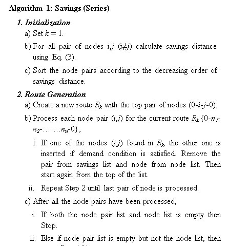
In series approach, if a customer pair does not match, it is skipped. Each time a customer is inserted into a route, one must start a new from the top of the list as the combinations that were not viable so far, now may have become viable. It creates one route at a time and requires several pass through the customer pair list. Algorithm 1 shows the steps of the series Savings.

The parallel version of Savings creates multiple partial routes at a time. When a pair of customer is processed, it is checked against all the routes already generated instead of only the current one. If a pair doesn’t matches, a new route is created with the pair, while it is skipped in series approach. After each insertion, the partial routes are considered for merging. In parallel Savings, only one pass requires through the savings pair list for route construction. The steps of the

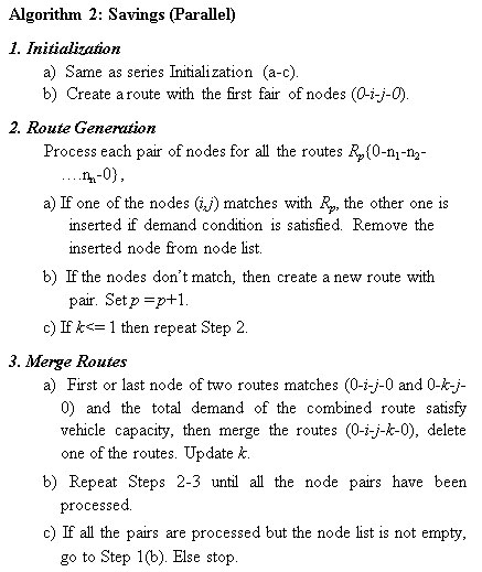
parallel Savings are shown in Algorithm 2.

Clustering Method

In clustering method, the solution of the problem is divided into two phases. All the nodes are grouped into several clusters using clustering algorithms and then the routes are optimized using any optimization technique. That’s why this approach is also known as 2-phase or cluster first, route second algorithm.

Sweep Algorithm

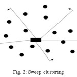
Sweep algorithm is the simplest clustering method for solving CVRP.^9,10 Cluster formation starts from 0⁰ and consequently advance towards 360⁰ to assign all the nodes under different vehicles while maintaining vehicle capacity. This type of sweeping is called forward sweep. And in backward sweep, clustering direction is clockwise which means though clustering starts from 0⁰, then it advances algorithm from 360⁰ to 0⁰. The general formula for calculating polar angle of the customers with respect to depot is,

θ =  tan^-1 (y/x)          (4)

θ = Angle of a node (depot/customer).

x, y = X, Y co-ordinates of customer.

Figure 2: Sweep clustering.  Click here to View figure

 

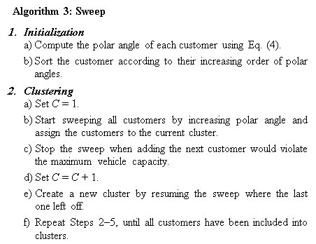
Figure 2 shows forward Sweep cluster creation starts from 0⁰ and goes in anti-clockwise direction. Algorithm 3 shows the Sweep steps.

Sweep Nearest Algorithm

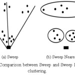
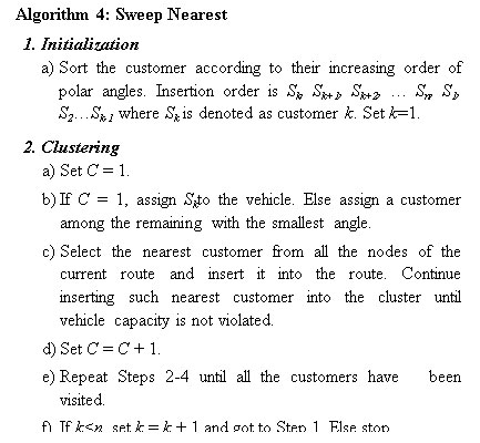
The Sweep algorithm clusters the nodes solely by polar angle. If the nodes are widely separated but have less angular difference, they may be grouped in the same cluster. This reduces the optimality of the solution cluster. To resolve this problem, an algorithm was proposed named Sweep Nearest algorithm (SN)¹⁵, which combines the classical Sweep and the Nearest Neighbor algorithm. SN first assigns a vehicle to the customer with the smallest polar angle among the remaining customers and then finds the nearest stop to those already assigned and then inserts that customer.

Figure 3 compares Sweep and Sweep Nearest clustering. Fig. 3(a) shows the clustering of Sweep algorithm where distant nodes are inserted into the same cluster due to their polar angle. On the other hand, closest nodes belong to the same cluster in Sweep Nearest as shown in Fig. 3(b) and produces better cluster. The procedure of Sweep Nearest algorithm is shown in Algorithm 4.

Figure 3: Comparison between Sweep and Sweep Nearest clustering.   Click here to View figure

 

Sweep Reference Point Algorithm

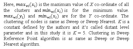
In the Sweep and Sweep Nearest, the depot is used as a reference point for calculating the polar angle. Changing the reference point alters the polar angle of nodes and the insertion sequence of nodes and causes different routes to be generated. Based on these observations, the authors of¹⁵ proposed two different kinds of reference points rather than the depot: every node and distant point.

Every Node as Reference Point

Polar angle of the customers is calculated with respect to the other customers except depot. The formula is,

where

x_j,y_j = X, Y co-ordinates of customer i.

x_r, y_r= X, Y co-ordinates of the reference node.

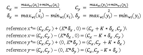
Distant Point as Reference Point

The distant reference points are denoted as x⁺, x^–, y⁺, y^–. They are calculated using the following formula,

Fisher and Jaikumar Algorithm

This algorithm¹¹ solves a Generalized Assignment Problem (GAP) to form the clusters. In GAP, there are a number of agents and a number of tasks. This problem is a generalization of the assignment problem in which both tasks and agents have a size. Moreover, the size of each task might vary from one agent to the other. Any agent can be assigned to perform any task, incurring some cost and profit that may vary depending on the agent-task assignment. Moreover, each agent has a budget and the sum of the costs of tasks assigned to it cannot exceed this budget. It is required to find an assignment in which all agents do not exceed their budget and total profit of the assignment is maximized. When GAP is applied for CVRP, the vehicles are considered as agents, vehicle capacity is agent’s budget, tasks are customers and profit is the optimal route cost. The assignment of customers to vehicles is done in such a way that vehicle capacity is not violated and the traveled distance is as less as possible.

Figure 4: Seed customer selection in Fisher and Jaikumar. Click here to View figure

 

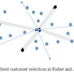
At first, in Fihser and Jaikumar algorithm, the customers are divided into K cones where K is the number of total vehicles. Seed customers are selected from the cones, based on some criteria such as customers with maximum demand or most distant customer from origin. Fig. 4 shows that the customers (N = 15) are divided into four cones (K = 4). If the smallest angle is 20⁰ and the largest angle is 340⁰ then each cone is of 80⁰. From each cone, the farthest node from the origin is chosen as the seed customer. After seed selection, insertion cost is calculated which is the cost of inserting customer within the route going back and forth between seed customer and depot. Then the customers are assigned to vehicles according to the increasing order of insertion cost.

Figure 5 demonstrates visiting seed and a customer where 0 denotes the depot, S is seed customer and i is the customer being considered for insertion. Fig. 5(a) shows the back and forth route of seed customer and depot. Fig. 5(b) shows the route if customer i is visited in the way of returning from seed customer to depot. From Fig. 5(a), the traveled distance d_S of visiting the seed customer and returning to depot is,

d_S = d_0S + d_S0= 2d_S                                                         (6)

And if customer i is visited on the way while visiting seed,

Figure 5: Demonstration of visiting seed alone and with a customer Click here to View figure

 

then the distance d_i,

d_i = d_S+ d_Si + d_i0                                                         (7)

Substituting Eq. (6) from Eq. (7), insertion cost of customer i is

C_ik= d_i – d_S= d_Si + d_i0 – d_S                     (8)

The authors of [11] pointed some attractive attributes of the algorithm. First, the heuristic is always find a feasible solution if one exists due to the characteristics of GAP. Second, when the GAP is solved, the algorithm is considering the impact of a customer assigned to a vehicle on every other possible assignment. This avoids a problem faced by sequential assignment or limited adjustment heuristics that is unknowingly making initial assignment which may lead to expensive route generation. Third, the method can be easily adapted to accommodate the constraints of CVRP. Finally, it lets to select seed customer and thus it helps in generating

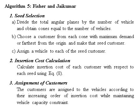
different route set. The procedure of Fisher and Jaikumar algorithm is shown in Algorithm 5.

Optimum Route Generation

The route generation stage is aimed to optimize searching method to find the optimal solution that represents the shortest path between all nodes in each cluster generated by the clustering algorithm. In this stage each cluster is an individual traveling salesman problem (TSP). In this study, three prominent methods are considered for route optimization: Genetic Algorithm (GA), Ant Colony Optimization (ACO) and Velocity Tentative Particle Swarm Optimization (VTPSO). GA is a prominent and pioneer optimization method. ACO is the prominent Swarm Intelligence (SI) based method and is pioneer in solving   TSP. On the other hand, Velocity Tentative Particle Swarm Optimization (VTPSO) is recently developed method extending PSO of continuous optimization. Brief description of the methods to optimize route (i.e., to solve TSP) are given to make the paper self-contained.

Genetic Algorithm (GA)

GA¹² is inspired by biological systems’ fitness improvement through evolution and is the pioneer and widely used to solve many scientific and engineering problems. Common features of GA are: populations of chromosomes (i.e., solutions), selection according to fitness, crossover to produce new offspring, and random mutation of new offspring. To produce new tour from existing tours, Enhanced Edge Recombination cross over method is used in this study. The positions of two nodes are interchanged for mutation operation.

Ant Colony Optimization (ACO)

ACO is inspired from ants’ foraging behavior and is the prominent method for solving TSP.^13,16 ACO is the first algorithm aiming to search for an optimal path in a graph, based on the behavior of ants seeking a path between their colony and a source of food. It considers population size as the number cities in a given problem and starts placing different ants in different cities. A particular ant consider next city to visit based on the visibility heuristic (i.e., inverse of distance)

and intensity of the pheromone on the path. After the completion of a tour, each ant lays some pheromone on the path. Before pheromone deposit, pheromone evaporation of real ant is adopted by reducing pheromone of all the links by a fixed percentage. This behavior allows the artificial ants to forget bad choices made in the past. Finally, all the ants follow the same route after certain iteration. The detail description of ACO is available in.¹⁹

Velocity Tentative PSO (VTPSO)

VTPSO¹⁴ is the most recent SI based method extending Particle Swarm Optimization (PSO) to solve TSP. In PSO, a particle represents a feasible solution in multi-dimensional search space. In each iteration, each particle measure its velocity considering its own past best position and the best position encountered by the whole swarm. VTPSO calculates velocity as Swap Sequence (SS) to alter a TSP solution to new one but apply the SS in a different and optimal way. A SS is a collection of Swap Operators (SOs) and each SO is a pair of indexes to alter. On the other hand, VTPSO considers the calculated velocity SS as tentative velocity and conceives a measure called partial search (PS) to apply calculated SS to update particle’s position (i.e., TSP tour). VTPSO measures tours with portions of SS and conceives comparatively better new tour with a portion or full tentative SS. The algorithm is described in.¹⁴

Experimental Studies

This section first describes the benchmark problems and experimental setup for conducting the experiment. Then it compares outcomes of different methods.

Benchmark Data and Experimental Setup

In this study, a suite of benchmark problem named Augerat et al., (A-VRP) has been chosen¹⁷ Each data set includes the number of customers, number of vehicles available and each vehicle capacity. A customer is represented as a two dimensional coordinate and individual customer demand is also given. In A-VRP, number of customer varies from 32 to 80, total demand varies from 407 to 932, and number of vehicle varies from 5 to 10. The capacity of individual vehicle is 100 for all the problems. The original data set is modified here to make the coordinate of the depot as (0, 0).

We strongly relied on an experimental methodology for configuring the route optimization algorithms. For the fair comparison, the number of iteration was set to 100 for the algorithms. The population size was 50 for GA and VTPSO. The number of ants in ACO was equal to the number of nodes in a cluster as it desired. In ACO, alpha and beta were set to 1 and 3, respectively. The selected parameters are not optimal values, but considered for simplicity as well as for fairness in observation.

The algorithms are implemented on Visual C++ of Visual Studio 2013. The experiments have been done on a PC (Intel Core i5-3470 CPU @ 3.20 GHz CPU, 4GB RAM) with Windows 7 OS.

Experimental Results and Analysis

This section presents experimental results for different clustering and route optimization methods. Route optimization is performed with GA, ACO and VTPSO for each clustering method. Table 1 shows the initial route cost and optimized route cost of Savings Series (SVS) and Savings Parallel (SVP) for benchmark problems. Table 2 is for optimized CVRP route cost of Sweep algorithm (SW), Sweep Nearest algorithm (SN), Sweep Reference Point algorithm using every stop (SRE), Sweep with Reference with Distant point (SRD) and Fisher and Jaikumar algorithm (FJ). From the tables, it can be observed that for the same instances and using same optimization technique, the route costs are different due to different approach of cluster/route generation. The best route found for each instance is shown as bold. On the other hand, in few cases a method requires an additional vehicle to cover all the nodes which are marked with a along with CVRP cost. It is observed from Table 1 that SVP is better than SVS. Without optimization, SVP is shown better CVRP cost than SVP for all the cases except n53-k7. In few cases outperformance of SVP is significant. For n33-k5 problem, as an example, SVS achieved CVRP cost 957 and SVP achieved 842. However, SVP involves more computation than SVS; SVP includes customer insertion and route merging.

Table 1 also presents effect of vehicle route optimization on both SVS and SVP. In general, optimization does not incur with Savings since it looks on overall CVRP cost while generating solutions. For better understanding, ‘-’ indicates optimization is not found effective for the instances. From the table it is found that ACO is unable to improve CVRP solution for any cases of SVP and SVS. GA is found to improve solutions 22 and 16 cases for SVS and SVP, respectively. On the other hand, VTPSO improved all 27 cases for SVS and 18 cases for SVP. 22 and all 27 cases. At a glance, solving CVRP with Savings, SVP + VTPSO is the best method. Finally, the interesting observation from the table is that there is a scope to improve Savings solution through TSP optimization methods.

Table 1: CVRP cost of Savings algorithms (Series and Parallel) for A-VRP benchmark problems. ‘-’ indicates optimization is not found effective for the problems. . ^a with cost indicates an additional vehicle was required to solve the problem.

		Without Optimization		Optimization with
				GA		ACO		VTPSO
		SVS	SVP	SVS	SVP	SVS	SVP	SVS	SVP
1	n32-k5	957	842	937	829	–	–	927	829
2	n33-k5	769	716	759	711	–	–	759	711
3	n33-k6	926	774a	916	–	–	–	916	–
4	n34-k5	886	809a	862	–	–	–	862	–
5	n36-k5	994	835	973	806	–	–	973	806
6	n37-k5	898	705	838	704	–	–	833	693
7	n37-k6	1061	977	1048	975	–	–	1048	975
8	n38-k5	847	770a	830	769a	–	–	827	–
9	n39-k5	1031	907	1020	–	–	–	1020	–
10	n39-k6	1024	857	997	855	–	–	992	855
11	n44-k6	1155	1006	1111	1005	–	–	1108	1005
12	n45-k6	1120	997a	1118	992a	–	–	1116	992a
13	n45-k7	1334	1198	1313	–	–	–	1311	–
14	n46-k7	1133	939	1045	937	–	–	1038	936
15	n48-k7	1234	1110	1214	–	–	–	1214	1100
16	n53-k7	1167	1198	–	1083	–	–	1146	1083
17	n54-k7	1379	1209	1361	1192	–	–	1361	1191
18	n55-k9	1277	1109	1274	–	–	–	1266	–
19	n60-k9	1638	1408	1616	1406	–	–	1614	1406
20	n61-k9	1302a	1058a	1286a	–	–	–	1282a	1050a
21	n62-k8	1622	1368	1603	–	–	–	1600	–
22	n63-k9	1904	1682a	–	1680a	–	–	1885	1678a
23	n63-k10	1556	1352	–	1345	–	–	1548	1342
24	n64-k9	1763	1489a	–	1488a	–	–	1701	1482a
25	n65-k9	1519	1266a	1500	–	–	–	1492	–
26	n69-k9	1312	1192	1195	–	–	–	1188	–
27	n80-k10	1967	1840	–	–	–	–	1955	1836
Best Count		0	7	0	10	0	0	1	18
Improvement due to optimization				22	16	0	0	27	18

 

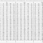Table 2: CVRP cost for different clustering and optimization methods for A-VRP benchmark problems. a with cost indicates an additional vehicle was required to solve the problem.   Click here to View table

 

Results presented in Table 2 for SW is for both forward and backward where anti-clockwise and clockwise sweep have been applied to form clusters. In SW, clusters are created based on solely customer’s angular position. One problem with polar angle clustering is customers separated widely may be inserted into the same cluster due to less angle difference. For this reason, Sweep Nearest (SN) was introduced which considers both angle and distance between customers to generate routes and thus produces better solution than SW. But in SN, for each insertion, distance between the clustered customers and remaining customers are computed for finding the nearest customer to insert. Also SN considers each customer as starting node and creates cluster set equal to the number of customers. As an example of n33-k5 problem, SN generates 33 clusters sets and selects the clusters set with the least CVRP cost. Thus SN requires more computation and iteration than SW and quite inefficient for large problem.

Results in Table 2 for Sweep Reference Point considered two different kind of reference points rather than depot; every stop (SRE) and distant points (SRD). It is notable that reference point is depot in SW and SN. For a particular optimization method (e.g., GA) the difference in outcome among SW, SN, SRE and SRD are due to reference point alteration. For instance n33-k5 problem, when the reference point is depot the CVRP costs after optimization with GA are 791 and 709 for SW and SN, respectively. But, when reference point changes, the cost reduced to 712 and 700 for GA for SRE and SRD, respectively. Similar effect for ACO and VTPSO are also observed. Various reference node increases the optimality of the clusters for many instances. SRD works with 4 reference points where SRE considers every node except customers. Therefore, SRE is shown better performance than SW, SN and SRD. With VTPSO optimization, SRE+VTPSO is shown best CVRP cost for 13 cases out of 27 cases.

From the Table 2 it is observed that Fisher and Jaikumar (FJ) with GA is shown to achieve best CVRP solutions for three cases n37-k5, n45-k7 and n61-k9. FJ selects distant customers as seed. Therefore, it considers farthest customers from depot for insertion at first and nearest ones later. The distant customers influences the cost of the clusters more than the nearest. Because the customers closer to depot can be inserted into any clusters and it will have less impact on the cost than the distant customers’ insertion. It performs better when the customers are evenly distributed around the depot. It creates all the clusters in parallel, considers the insertion of a customer in all the cluster and inserts into the best suitable one. But customer density may vary in different regions; thus seed selection influences optimality of the routes. In some angular area customers may not even exists. When the customers are densely located in a particular area, more seeds get selected from that area comparing with the other areas. SW and SN outperform FJ for most of the instances. But FJ also produces feasible clusters (where cluster number does not exceed the vehicles provided) and involves less computation time.

Considering results of Table 1 and Table 2, after implementing different optimization techniques, the CVRP costs do not vary for constructive algorithm as much as for clustering algorithm. Also Savings algorithm (Table 1) is

giving same result for different optimization algorithms. On the other hand, for clustering algorithm GA is performing better than ACO; and VTPSO is outperforming both GA and ACO. Among 27 instances, VTPSO is giving best result for 22 cases.

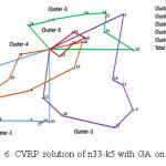
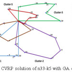
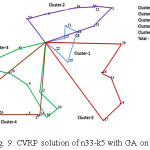
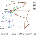
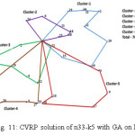
Figures 6 to 11 show graphical representation of final CVRP solutions with route optimization with GA for SVS, SVP, SW, SN, SRD and FJ for sample problem n33-k5. Fig. 6 and Fig. 7 demonstrate the CVRP solutions for SVS and SVP, respectively. Common feature of SVS and SVP is that both contains intersections clusters. On the other hand, clusters are varied in the two method with different nodes. Node 24 is in cluster 3 in SVS and in Cluster 5 in SVP. Total CVRP costs for SVS and SVP are 759 and 711, respectively.      

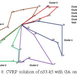
Figure 8 shows the CVRP solution for SW+GA. There is no intersection in clusters in the route. SW clustering starts from a particular angle and advances only either forward or backward; thus there is no scope of intersection. Although routes of individual looks nice but CVRP cost is relatively high and is 791.

Figure 6: CVRP solution of n33-k5 with GA on SVS.  Click here to View figure

 

Figure 7: CVRP solution of n33-k5 with GA on SVP.  Click here to View figure

 

Figure 8: CVRP solution of n33-k5 with GA on SW Click here to View figure

 

Figure 9 and Fig. 10 demonstrate the CVRP solutions for two SW variants SN and SRD, respectively. Common feature of the methods is cluster intersections. In the methods cluster formation varies due to reference point’s variation. On the other hand, clusters are varied in the two method with different nodes. The CVRP cost of the methods are promising and achieved cost of 700 by SRD is the best among the methods with GA. Finally, Fig. 11 shows the solution with FJ which is similar to SRD. Hence, CVRP cost of FJ is also competitive to SRD and achieved value is 705.

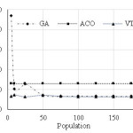
There is an effect of population size on performance in any population based method. For better understanding, the effect of population size is investigated for GA and VTPSO varying population size from 5 to 200. The population size in ACO was the number nodes in a particular cluster. While varying population, the number of generation was fixed at 100. Fig. 12 shows CVRP route costs on SW based clusters of n62-k8 problem. From the figure it is observed that performance of GA is highly dependent on population size. It showed very bad CVRP cost for very small population (e.g., 5) and became steady for population with 50 or more. VTPSO also found population dependent but performed relatively better for small population. At a glance, VTPSO outperformed both GA and ACO.

Figure 9: CVRP solution of n33-k5 with GA on SN  Click here to View figure

 

Figure 10: CVRP solution of n33-k5 with GA on SRD.  Click here to View figure

 

Figure 11: CVRP solution of n33-k5 with GA on FJ  Click here to View figure

 

Figure 12 Click here to View figure

 

Conclusion

CVRP is a popular combinatorial optimization problem and interest grows in recent years to solve it new ways. Two popular ways of solving CVRP are constructive and clustering methods. Constructive method based algorithms create routes and minimize the cost at the same time. On the other hand, clustering algorithms require two phase to get an optimal solution. Constructive algorithms do not consider alternate solutions. Also constructive method performs better than clustering in most of the instances. Finally, GA, ACO and VTPSO are applied to generate optimal route with the both constructive and clustering algorithms’ outcome. Although optimization technique generally not consider constructive approach, this study revealed that there is a scope to improve Savings solution through TSP optimization methods. Among the three route optimization methods, VTPSO is shown the best and performed well with SVP and SRE.

Conflict of Interest

Authors declared that there is no conflict of interest.

References

1. G. B. Dantzig and J. H. Ramser. “The Track Dispatching Problem.” INFORMS, Management Science.1959;6(1):80-91.
   CrossRef
2. Christofides N, Mingozzi A, Toth P. “The vehicle routing problem”, In: Christofides N, Mingozzi A, Toth P, Sandi C, editors.
3. S. R.Venkatesan, D. Logendran, D. Chandramohan. “Optimization of Capacitated Vehicle Routing Problem using PSO.” International Journal of Engineering Science and Technology (IJEST).2011;3:7469-7477.
4. Jens Lysgaard, “Clarke & Wright’s Savings Algorithm”, Department of Management Science and Logistics, the Aarhus School of Business1997.
5. A. Poot & G. Kant. “A Savings Based Method for Real-Life Vehicle Routing Problems.” Econometric Institute Report EI 9938/A, August 1, 1999.
6. T. Doyuran, B. Çatay. “A robust enhancement to the Clarke-Wright savings algorithm.” Technical notes, Faculty of Engineering and Natural Sciences, Sabanci University, Tuzla, Istanbul, Turkey, 2011.
   CrossRef
7. T. Pichpibula, R. Kawtummachai. “An improved Clarke and Wright savings algorithm for the capacitated vehicle routing problem”, Science Asia, vol. 38, pp. 307–318, 2012.
   CrossRef
8. B. E. Gillet and L. R. Miller. “A Heuristic Algorithm for the Vehicle Dispatch Problem.” Operations Research.1974;22:340-349.
   CrossRef
9. G. W. Nurcahyo, R. A. Alias, S. M. Shams uddin and M. N. Md. Sap. “Sweep Algorithm in vehicle routing problem for public Transport.” Journal Antarabangsa (Teknologi Maklumat).2002;2:51-64.
10. N. Suthikarnnarunai. “A Sweep Algorithm for the Mix Fleet Vehicle Routing Problem.” In Proceedings of the International Multi-Conference of Engineers and Computer Scientists 2008 Vol II, IMECS 2008, 19-21 Hong Kong, March 2008.
11. M. L. Fisher and R. Jai kumar. “A Generalized Assignment Heuristic for Vehicle Routing.” Networks.1981;11:109-124, 1981.
    CrossRef
12. D. E. Goldberg. “Genetic Algorithm in Search, Optimization and Machine Learning.” New York: Addison – Wesley, 1989.
13. T. Stutzle and M. Dorigo. “The Ant Colony Optimization Metaheuristic: Algorithms, Applications, and Advances.” International Series in Operations Research and Management Science. Kluwer, 2001.
14. M. A. H. Akhand, S. Akter, M. A. Rashid and S. B. Yaakob. “Velocity Tentative PSO: An Optimal Velocity Implementation based Particle Swarm Optimization to Solve Traveling Salesman Problem.” IAENG International Journal of Computer Science.2015;42(3):221-232.
15. Byungsoo Na, Yeowoon Jun & Byung-In Kim.“Some extensions to the sweep algorithm.” Int J Adv Manuf Technol.2011;56:1057–1067.
    CrossRef
16. Y. F. Liao, D. H. Yau and C. L. Chen. “Evolutionary Algorithm to Traveling Salesman Problems,” Computers & Mathematics with Applications.2012;64(5):788–797.
    CrossRef
17. Large Capacitated Vehicle Routing Problem Instances. Available: http://neo.lcc.uma.es/vrp/vrp-instances/.

---

This work is licensed under a Creative Commons Attribution 4.0 International License.