S. P. Sajjan1, Ravi kumar Roogi1, Vijay kumar Badiger1, Sharanu Amaragatti2
1Research Scholar Dept. of Computer Science Ku, Dharwad
2Software Engineer Consonant consulting india itd,pvt Banglore
Article Publishing History
Article Received on :
Article Accepted on :
Article Published :
Article Metrics
ABSTRACT:
This paper introduces a well known NP- Complete problem called the Knapsack Problem, presents several algorithms for solving it, and compares their performance. The reason is that it appears in many real domains with practical importance. Although it’s NP-Completeness, many algorithms have been proposed that exhibit impressive behaviour in the average case. This paper introduce A New approach to solve a Knapsack Problem. An overview of the previous research and the most known algorithms for solving it are presented. The paper concludes with a practical situation where the problem arises.
KEYWORDS:
This paper introduces; New Approach To
Copy the following to cite this article:
Sajjan S. P, Roogi R. K, Badiger V. K, Amaragatti S. A New Approach To Solve Knapsack Problem. Orient. J. Comp. Sci. and Technol;7(2)
|
Copy the following to cite this URL:
Sajjan S. P, Roogi R. K, Badiger V. K, Amaragatti S. A New Approach To Solve Knapsack Problem. Orient. J. Comp. Sci. and Technol;7(2). Available from: http://www.computerscijournal.org/?p=1254
|
Introduction
Many people wants to fill up his knapsack, selecting among various objects. Each object has a particular weight and obtains a particular profit. The knapsack can be filled up to a given maximum weight. How can he choose objects to fill the knapsack maximizing the obtained profit?
A naïve approach to solve the problem could be the following
Select each time the object which has the highest profit and fits in the knapsack, until you can’t choose any more objects.
Unfortunately, this algorithm gives a good(or bad)_ solution which, in general isn’t optimal. This is the case also if you try other rules, such as “ choose the object with the highest ratio profit/weight”, As a result, you may not do anything else, other than testing all the possible subset of chosen objects. Note that for n objects there are 2n such subsets.
The simple problem above is in fact an informal version of an important and famous problem called The Knapsack Problem. This paper studies the problem from the point of view of theoretical Computer Science.
The Problem
The Knapsack Problem belongs to a large class of problems known as Combinatorial Optimization Problem. In such problem, we try to “Maximize” (or “Minimize”) some “ Quantity”, while satisfying some constraints. For example, the Knapsack problem is to maximize the obtained profit without exceeding the knapsack capacity. In fact, it is a very special case of the well-known Integer Linear Programming Problem.
Definition
Knapsack problem is defined as “It is a greedy method in which knapsack is nothing but a bag which consists of n objects each objects an associated with weight and profit”.
Objective: “To fill the knapsack to which maximum profits obtained”.
Formula
Let m be the capacity of knapsack
Let Xi be the solution vector.
Maximise = ∑1≤i≤nPiXi ———– (1)
Subject to
Maximise = ∑1≤i≤nWiXi ≤ m ———– (2)
Constraints
0 ≤ i ≤ n & 0 ≤ Xi ≤ n ———– (3)
where
Pi & Wi are the profit & weight are positive Numbers
- Equation (2) and (3) are satisfy the feasible solution i.e solution satisfy all the constraints
- Equation (1) is used to maximise the profit then it given optimal solution. i.e Best solution among all feasible solution.
Algorithm: knapsack(m,n)
Purpose: Gready method to solve knapsack problem
Input: m, n
Output: Xi→ àSolution vector
{
for i=1 to n
{
X[i] = 0.0;
U= m;
for i = 1 to n
{
if(w[i] > U)
break;
X[i] = 1.0;
U = U- W[i];
}
if(i n)
X[i] = U/W[i];
}
}
Knapsack Problem
Problem No 1:
Given n =3 m=20
(P1,P2,P3) = (25, 24, 15)
(W1, W2, W3) = (18, 15, 10)
Solution
Given problem can be solved by knapsack problem with Gready method as shown below
- Given n=3 then it has (n+1) feasible solution so given problem n has 3 then it contain (n+1) i.e 4 solutions.
- Out of 4 solutions we will solve given problem by using assumptions and algorithms.
- Given problem can be solved by 2 assumptions and 2 algorithms based.
( X1, X2, X3) ∑1≤i≤nWiXi ∑1≤i≤nPiXi
- (1/2, 1/3, 1/4) 16.5 24.2
- (1, 2/15, 0) 20 28.2
- (0, 2/3, 1) 20 31
- (0, 1, 1/2) 20 31.5
n = 3 Then (n+1) Solution → 4 solution
First solution: Based on Assumption
n = 4 1, 2, 3, 4
Divede one by remaining numbers i.e 1/2 1/3 1/4
Calculate corresponding weight and profit
∑1≤i≤nWiXi = (18*1/2 + 15*1/3 + 10*1/4)
= (9 + 5 + 2.5)
=16.5
∑1 ≤j≥ Pj Xj = (25*1/2 + 24*1/3 + 15*1/4)
= (12.5 + 8 + 3.7)
=24.2
Second Solution : Based on Algorithm
Algorithm: knapsack(m,n)
{
for i = 1 to n
X[i] = 0.0;
U =m;
for i = 1 to n
{
if( W[i] > U)
break;
X[i] = 1.0;
U = U-W[i];
}
if(i≤ n )
{
X[i] = U/W[i];
}
}
For given problem it check in algorithm then assign values
For X[i] X[2] X[3]
X[1] = 1
X[2] = 2/15
X[3] = 0
Then calculate corresponding weight and profit
∑1≤i≤nWiXi = (1*18 + 2/15*15 + 0*10)
= (18 + 2 + 0)
=20
∑1≤i≤nPiXi = (1*25 + 2/15*24 + 0* 15)
= (25+3.2)
=28.2
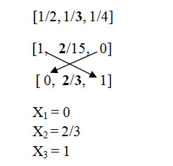
Third Solution: Based on Assumption
- Interchange the right most element to left most position & left most element to right most position
- In second middle element can be find take numerator of that element then we get values for third solution
Calculate corresponding weight & profit
∑1≤i≤nWiXi = (0*18 + 2/3*15 + 1*10)
= (10+10)
=20
∑1≤i≤nPiXi = (0*25 + 2/3*24 + 1*15)
= (16+15)
=31
Fourth Solution: Based on algorithms
For X[1] put 0 as value because its value is already find in second solution then start with X[2].
X[1] = 0
X[2] = 1
X[3] = 5/10 = 1/2
Then calculate corresponding weight and Profit
∑1≤i≤nWiXi = (0*18 + 1*15 + 1/2*10)
= (15+5)
=20
∑1≤i≤nPiXi = (0*25 + 1*24 + 1/2*15)
= (24+7.5)
=31.5
Based on Second method (Based on Algorithm) we got profit 28.2, but acourding to our Assumption we got profit 31, this is better solution as compare second method, unfortunately Third method not an optimal solution, If you apply again Algotithm based on second method assuption we got profit 31.5, Fourth solution answer near to our Third Assumption method.
Among Four feasible solutions the solution 4 obtained the maximum profit so that fourth solution is Optimal Solution for this problem.
Analysis
- If the items are already sorted into decreasing order of Vi / Wi, then time complexity is O(n).
- Therefore Time Complexity including sort is O(n log n)
Conclusion
In this paper we proposed an algorithm to solve the knapsack problem. This algorithm originates from a well-known continued fraction method and runs in polynomial time of the input lengh. We conjecture that for any fixed n>2, the knapsack problem with n variables may be solved in polynomial time. The proof seems difficult and generalization of the method used in this paper doesn’t seem to work. It is hoped that the modest beginning presented in this paper will draw the attention of more researchers and will bring about the eventual solution of this problem.
References
- Horowitz, E and Sahni, S.Computing partitions with applications to the knapsack problem J ACM 21, 2(April 1974), 277-292.
CrossRef
- Prof S. Nandagopalan, Analysis and Design of Algorithms,112-114.
- A.M. Padma Reddy,”Desgin and analysis of algorithms 6th Edition”, 2012.
- The T emporal Knapsack Problem and Its Solution Mark Bartlett, Alan M. F risch, Youssef Hamadi, Ian Miguel, S. Armagan T arim, and Chris Unsworth.
- A Polynomial-Time Algorithm for the Knapsack Problem with Two Variables D. S. HIRSCHBERG AND C. K. WONG, Journal of the Assacmtion for Computing Machinery, Vol 23, No 1, January 1976.
- The 0–1 Knapsack Problem An Introductory Survey Michail G. Lagoudakis.

This work is licensed under a Creative Commons Attribution 4.0 International License.